Page 191 - Fundamentals of Radar Signal Processing

(3.11)

and is within the plausible maximum detection range of the radar. Note that n =
0 for target #1 and n = 1 for target #2 in the example of Fig. 3.6. Techniques to
deal with range and Doppler ambiguities are discussed in Chap. 5.

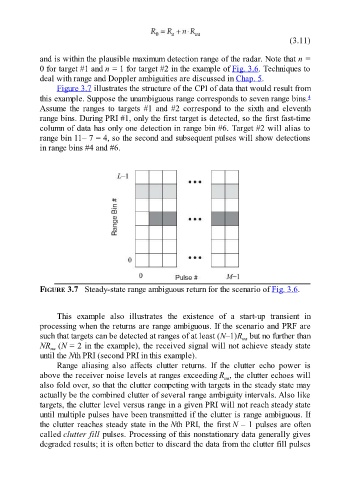
Figure 3.7 illustrates the structure of the CPI of data that would result from
this example. Suppose the unambiguous range corresponds to seven range bins. 4
Assume the ranges to targets #1 and #2 correspond to the sixth and eleventh
range bins. During PRI #1, only the first target is detected, so the first fast-time
column of data has only one detection in range bin #6. Target #2 will alias to

range bin 11– 7 = 4, so the second and subsequent pulses will show detections
in range bins #4 and #6.

FIGURE 3.7 Steady-state range ambiguous return for the scenario of Fig. 3.6.

This example also illustrates the existence of a start-up transient in
processing when the returns are range ambiguous. If the scenario and PRF are
such that targets can be detected at ranges of at least (N–1)R but no further than
ua
NR (N = 2 in the example), the received signal will not achieve steady state
ua
until the Nth PRI (second PRI in this example).
Range aliasing also affects clutter returns. If the clutter echo power is

above the receiver noise levels at ranges exceeding R , the clutter echoes will
ua
also fold over, so that the clutter competing with targets in the steady state may
actually be the combined clutter of several range ambiguity intervals. Also like
targets, the clutter level versus range in a given PRI will not reach steady state
until multiple pulses have been transmitted if the clutter is range ambiguous. If
the clutter reaches steady state in the Nth PRI, the first N – 1 pulses are often
called clutter fill pulses. Processing of this nonstationary data generally gives

degraded results; it is often better to discard the data from the clutter fill pulses