Page 287 - Fundamentals of Radar Signal Processing

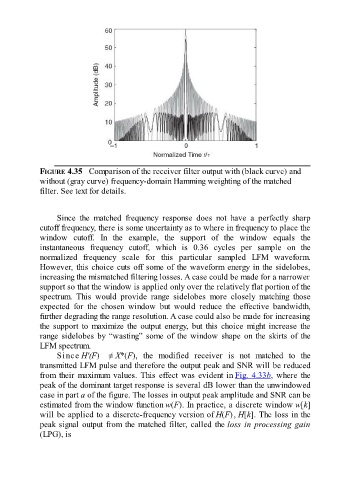
FIGURE 4.35 Comparison of the receiver filter output with (black curve) and
without (gray curve) frequency-domain Hamming weighting of the matched
filter. See text for details.

Since the matched frequency response does not have a perfectly sharp
cutoff frequency, there is some uncertainty as to where in frequency to place the
window cutoff. In the example, the support of the window equals the

instantaneous frequency cutoff, which is 0.36 cycles per sample on the
normalized frequency scale for this particular sampled LFM waveform.
However, this choice cuts off some of the waveform energy in the sidelobes,
increasing the mismatched filtering losses. A case could be made for a narrower
support so that the window is applied only over the relatively flat portion of the
spectrum. This would provide range sidelobes more closely matching those
expected for the chosen window but would reduce the effective bandwidth,

further degrading the range resolution. A case could also be made for increasing
the support to maximize the output energy, but this choice might increase the
range sidelobes by “wasting” some of the window shape on the skirts of the
LFM spectrum.
Since H′(F) ≠ X*(F), the modified receiver is not matched to the
transmitted LFM pulse and therefore the output peak and SNR will be reduced

from their maximum values. This effect was evident in Fig. 4.33b, where the
peak of the dominant target response is several dB lower than the unwindowed
case in part a of the figure. The losses in output peak amplitude and SNR can be
estimated from the window function w(F). In practice, a discrete window w[k]
will be applied to a discrete-frequency version of H(F), H[k]. The loss in the
peak signal output from the matched filter, called the loss in processing gain
(LPG), is