Page 335 - Fundamentals of Radar Signal Processing

way antenna power gain, and accounted for receiver noise, clutter cell size and

power variation with range, and other factors. The resulting range-Doppler
clutter spectrum, not including any aliasing in range or Doppler due to the PRF,
is shown in Fig. 5.4. Part a of the figure gives a 3D view, while part b is shows
a perhaps more useful 2D view. It is readily seen that the maximum clutter
power occurs at the mainlobe peak, centered at 93.4 m/s and 17.3 km. The high
antenna sidelobes (no weighting was used) create visible rings of clutter power

around the mainlobe. The shortest-range clutter occurs at zero velocity and just
over 3 km; this is the altitude line, and it is also relatively strong. It can be seen
that at any longer range, which must be at some angle other than directly below
the radar, the clutter must have a nonzero velocity, so the clutter energy spreads
to the maximum relative velocities of ±134.1 m/s (Doppler shifts of ±89.4 kHz)
as the range increases. In these figures, positive velocities (Doppler shifts) must
come from clutter in front of the aircraft, while negative velocities come from

clutter behind the aircraft. Figure 5.4c of the figure show the total clutter power
versus range, integrated over velocity. This illustrates the high AL return, the
fall-off of the clutter with range, and the large MLC return before the clutter
falls off again. Figure 5.4d shows the power versus velocity, integrated over
range, and illustrates the MLC, the relatively strong AL and the falloff at higher
velocities, which imply greater cone angle, longer ranges, and shallower

grazing angles with attendant lower clutter reflectivity.
These examples only hint at the complexity of the range-Doppler spectrum.
The subject will be revisited in Sec. 5.3 as part of the discussion of pulse
Doppler processing. Despite the potential complexity, the simple spectrum of
Fig. 5.1c has all the features needed to introduce MTI.

5.2 Moving Target Indication
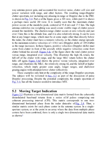
Figure 5.5 illustrates a two-dimensional data matrix formed from the coherently

demodulated baseband returns from a series of M pulses comprising one
coherent processing interval (CPI). This matrix corresponds to one two-
dimensional horizontal plane from the radar datacube of Fig. 3.8. Thus, a
similar matrix exists for each phase center in the antenna system. In a single-
aperture system, or at the point in an array where the data from multiple phase
centers have been combined, there is only a single two-dimensional data matrix

as shown. 2