Page 346 - Fundamentals of Radar Signal Processing

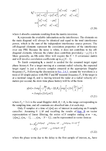
(5.20)

where k absorbs constants resulting from the matrix inversion.
S represents the available information on the interference. The elements on
I
the main diagonal will always be identical and equal to the total interference
power, which is the sum of the independent interference source powers. The
off-diagonal elements represent the correlation properties of the interference
over one PRI. Because the noise is white, it does not contribute to the off-
diagonal elements, whereas the clutter does contribute provided ρ = ρ [1] ≠ 0.
c
More generally, an Nth order filter will require the N × N covariance matrix
and will involve correlation coefficients up to ρ [N – 1].
c
To finish computing h, a model is needed for the assumed target signal
phase history t. For a target moving at a constant radial velocity, the expected
target signal is just a discrete complex sinusoid at the appropriate Doppler
frequency F . Following the discussion in Sec. 2.6.3, assume the waveform is a
D
train of M simple pulses with PRI T and RF transmit frequency F. If the target is
t
at a nominal range R and is moving toward the radar at a radial velocity of v
0
meters per second, the slow-time phase history will be of the form

(5.21)

where F = 2v/λ is the usual Doppler shift, R ≈ R is the range corresponding to
s
D
0
the sampling time, and all constants are absorbed into A at each step.
Only N samples at a time of y[m] are of interest in analyzing an N-sample
canceller. Assuming N ≤ M and recalling the results of App. B on vector
representation of linear filtering, the series of N samples ending at m = m ,
0
{y[m ], y[m – 1], …, y[m – N + 1]}, can be represented in vector form as
0
0
0

(5.22)

where the phase terms due to the delay to the first sample of interest, m , have
0