Page 347 - Fundamentals of Radar Signal Processing

been absorbed into A and the signal has been renamed t to emphasize that it is
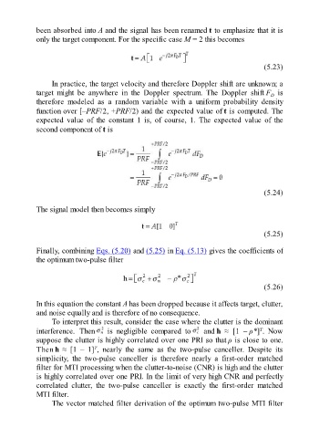
only the target component. For the specific case M = 2 this becomes

(5.23)

In practice, the target velocity and therefore Doppler shift are unknown; a

target might be anywhere in the Doppler spectrum. The Doppler shift F is
D
therefore modeled as a random variable with a uniform probability density
function over [–PRF/2, +PRF/2) and the expected value of t is computed. The
expected value of the constant 1 is, of course, 1. The expected value of the
second component of t is

(5.24)

The signal model then becomes simply

(5.25)

Finally, combining Eqs. (5.20) and (5.25) in Eq. (5.13) gives the coefficients of
the optimum two-pulse filter

(5.26)

In this equation the constant A has been dropped because it affects target, clutter,
and noise equally and is therefore of no consequence.

To interpret this result, consider the case where the clutter is the dominant
T
interference. Then is negligible compared to and h ≈ [1 – ρ*] . Now
suppose the clutter is highly correlated over one PRI so that ρ is close to one.
T
Then h ≈ [1 – 1] , nearly the same as the two-pulse canceller. Despite its
simplicity, the two-pulse canceller is therefore nearly a first-order matched

filter for MTI processing when the clutter-to-noise (CNR) is high and the clutter
is highly correlated over one PRI. In the limit of very high CNR and perfectly
correlated clutter, the two-pulse canceller is exactly the first-order matched
MTI filter.
The vector matched filter derivation of the optimum two-pulse MTI filter