Page 447 - Fundamentals of Radar Signal Processing

The idea of a sufficient statistic is quite rich. For example, it can be

interpreted as a geometric coordinate transformation chosen to place all of the
useful information in the first coordinate (Van Trees, 1968). Procedures for
verifying that a statistic (a function of the data y) is sufficient are given in Kay
(1993), as is the Neyman-Fisher factorization theorem for identifying sufficient
statistics. Detailed consideration of the properties of sufficient statistics is

beyond the scope of this text; the reader is referred to the references for greater
depth.
The specific value of the threshold η = –λ that will ensure that P = α as
FA
desired has not yet been found. The original expression for P was given in Eq.
FA
(6.2), but this is not very useful since its evaluation requires the N-dimensional
joint PDF of y and an explicit definition of the region , which have been
1
defined only implicitly as the points in N-space for which the LRT exceeds the

still-unknown threshold. Since they are functions of the random data y, Λ and ϒ
are also random variables and thus have their own probability density functions.
An alternate approach to computing the LRT threshold is thus to express P in
FA
terms of Λ or ϒ and then solve those expressions for η or equivalently for T.
The required expressions are

(6.15)

or

(6.16)

Because false alarms are the result of interference and do not involve targets,
the result depends only on the PDF of the likelihood ratio [if using Eq. (6.15)]
or the sufficient statistic [if using Eq. (6.16)] when a target is not present. Given
a specific model of that PDF, a specific value can be computed for η
(equivalently, λ or T.
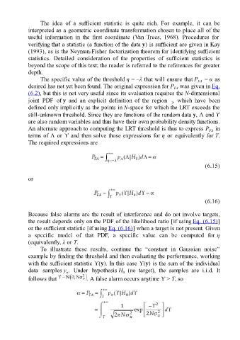
To illustrate these results, continue the “constant in Gaussian noise”
example by finding the threshold and then evaluating the performance, working

with the sufficient statistic ϒ(y). In this case ϒ(y) is the sum of the individual
data samples y . Under hypothesis H (no target), the samples are i.i.d. It
n
0
follows that . A false alarm occurs anytime ϒ > T, so