Page 450 - Fundamentals of Radar Signal Processing

(6.25)

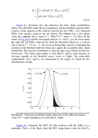
Figure 6.1 illustrates how the detection and false alarm probabilities

follow from the PDFs under the two hypotheses and the threshold, and how their
relative values depend on the relation between the two PDFs. Two Gaussian
PDFs with variance equal to one are shown. The leftmost has a zero mean,
while the rightmost has a mean of 1. With and m = 1/N these fit the
model of Eq. (6.9) and the subsequent analysis. P and P are the areas under
D
FA
the right and left PDFs, respectively, from the threshold (shown as a vertical
line at about ϒ = 1.5) to + ∞. The receiver design thus consists of adjusting the
position of the threshold until the black area equals the acceptable false alarm
probability. The detection probability is then the gray area (which includes the
black area). This figure again makes it clear that P and P must increase or
D
FA
decrease together as the threshold moves lower or higher. The achievable
combinations of P and P are determined by the degree to which the two
FA
D
distributions overlap.

FIGURE 6.1 Gaussian probability density functions of the sufficient statistic
when under hypothesis H (left) and H (right).
0
1

Figure 6.2 illustrates the ROC for this problem with the SNR χ as a
parameter. Part a of the figure plots the ROC using linear scales for both P FA