Page 529 - Fundamentals of Radar Signal Processing

Note that this procedure is effectively SOCA CFAR when the CUT is in the low

clutter region, and GOCA CFAR when it is in the high clutter region (assuming
the transition point is correctly located).
The discussion above does not allow for the possibility that the clutter is
uniform. To address this an additional likelihood test is conducted to compare
ln Λ(M ) as computed in Eq. (6.170) with M = M to the corresponding metric
t
t
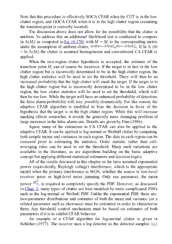
under the assumption of uniform clutter, . If ln Λ (0)
> ln Λ(M ) the clutter is assumed homogeneous and conventional CA CFAR is
t
applied.
When the two-region clutter hypothesis is accepted, the estimate of the
transition point M can of course be incorrect. If the target is in fact in the low
t
clutter region but is incorrectly determined to be in the high clutter region, the
high clutter statistics will be used to set the threshold. There will then be an
increased probability that the high clutter will mask the target. If the target is in

the high clutter region but is incorrectly determined to be in the low clutter
region, the low clutter statistics will be used to set the threshold, which will
then be too low. While the target will have an enhanced probability of detection,
the false alarm probability will rise, possibly dramatically. For this reason, the
adaptive CFAR algorithm is modified to bias the decision in favor of the
hypothesis that the target is in the high clutter region. While this will increase

masking effects somewhat, it avoids the generally more damaging problem of
large increases in the false alarm rate. Details are given by Finn (1986).
Again, many of the extensions to CA CFAR can also be applied to the
adaptive CFAR. It can be applied to log normal or Weibull clutter by computing
both sample means and variances in each region. The data in each region can be
censored prior to estimating the statistics. Order statistic rather than cell-
averaging rules can be used to set the threshold. Many such variations are

available in the literature, as are algorithms building on the basic adaptive
concept but applying different statistical estimators and decision logics.
All of the results discussed in this chapter so far have assumed exponential
power (equivalently, Rayleigh voltage) interference, which is the appropriate
model when the primary interference is WGN, whether the source is low-level

receiver noise or high-level noise jamming. Only one parameter, the mean
power , is required to completely specify the PDF. However, as discussed

in Chap. 2, many types of clutter are best modeled by more complicated PDFs
such as the log-normal or Weibull PDF. Unlike the exponential PDF, these are
two-parameter distributions and estimates of both the mean and variance (or a
related parameter such as skewness) must be estimated in order to characterize
them. Any threshold control mechanism must be based on estimates of both

parameters if it is to exhibit CFAR behavior.
An example of a CFAR algorithm for log-normal clutter is given in
Schleher (1977). The receiver uses a log detector so the detected samples {x }
i