Page 527 - Fundamentals of Radar Signal Processing

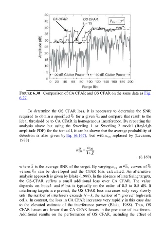
FIGURE 6.30 Comparison of CA CFAR and OS CFAR on the same data as Fig.

6.27.

To determine the OS CFAR loss, it is necessary to determine the SNR

required to obtain a specified for a given and compare that result to the
ideal threshold or to CA CFAR in homogeneous interference. By repeating the
analysis above but using the Swerling 1 or Swerling 2 model (Rayleigh
amplitude PDF) for the test cell, it can be shown that the average probability of
detection is also given by Eq. (6.167), but with α replaced by (Levanon,
OS
1988)

(6.169)

where is the average SNR of the target. By varying α or , curves of
OS
versus can be developed and the CFAR loss calculated. An alternative
analysis approach is given by Blake (1988). In the absence of interfering targets,
the OS-CFAR suffers a small additional loss over CA CFAR. The value
depends on both k and N but is typically on the order of 0.3 to 0.5 dB. If
interfering targets are present, the OS CFAR loss increases only very slowly

until the number of interferers exceeds N – k, the number of “ignored” high-rank
cells. In contrast, the loss in CA CFAR increases very rapidly in this case due
to the elevated estimate of the interference power (Blake, 1988). Thus, OS
CFAR losses are lower than CA CFAR losses in the presence of interferers.
Additional results on the performance of OS CFAR, including the effect of