Page 155 - Fundamentals of Reservoir Engineering

MATERIAL BALANCE APPLIED TO OIL RESERVOIRS 94

the reservoir, for the same aquifer volume, than for a linear aquifer and, as a result,
response of the radial aquifer is greater causing deviation below the theoretical straight
line. Exercise 9.2 provides an example of this technique in which the aquifer model
used for calculating W e caters for time dependence.

Once a satisfactory aquifer model has been obtained by history matching, the same
model can hopefully be used in predicting reservoir performance for any scheduled
offtake policy. As already mentioned, however, there are so many uncertainties
involved that the aquifer model is hardly ever unique and its validity should be
continually checked as fresh production and pressure data become available.

If the reservoir has a gascap then equ. (3.12) has the form

F = N (E o + mE g) + W e

which can alternatively be expressed as

F W
= N+ e (3.29)
(E + mE ) (E + mE )
g
g
o
o
in which it is assumed that both m and N are known.
By plotting F/(E o + mE g) versus W e /(E o + mE g) the interpretation is similar to that
shown in fig 3.9.

Equation (3.29) demonstrates how the technique of Havlena and Odeh can be applied
to a combination drive reservoir in which there are three active mechanisms, solution
gas drive, gascap drive and water drive.

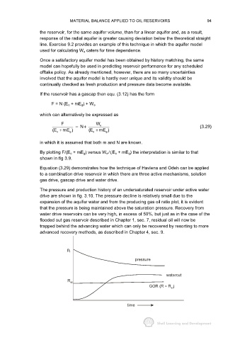
The pressure and production history of an undersaturated reservoir under active water
drive are shown in fig. 3.10. The pressure decline is relatively small due to the
expansion of the aquifer water and from the producing gas oil ratio plot, it is evident
that the pressure is being maintained above the saturation pressure. Recovery from
water drive reservoirs can be very high, in excess of 50%, but just as in the case of the
flooded out gas reservoir described in Chapter 1, sec. 7, residual oil will now be
trapped behind the advancing water which can only be recovered by resorting to more
advanced recovery methods, as described in Chapter 4, sec. 9.

p i

pressure

watercut
R si
GOR (R ≈ R )
si

time