Page 150 - Fundamentals of Reservoir Engineering

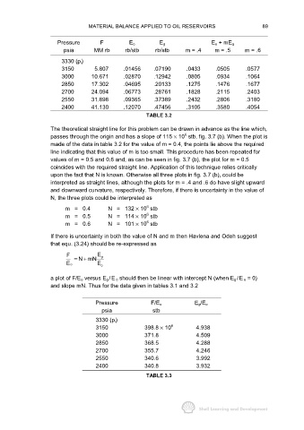
MATERIAL BALANCE APPLIED TO OIL RESERVOIRS 89

Pressure F E o E g E o + mE g
psia MM rb rb/stb rb/stb m = .4 m = .5 m = .6
3330 (p i)
3150 5.807 .01456 .07190 .0433 .0505 .0577
3000 10.671 .02870 .12942 .0805 .0934 .1064
2850 17.302 .04695 .20133 .1275 .1476 .1677
2700 24.094 .06773 .28761 .1828 .2115 .2403
2550 31.898 .09365 .37389 .2432 .2806 .3180
2400 41.130 .12070 .47456 .3105 .3580 .4054

TABLE 3.2

The theoretical straight line for this problem can be drawn in advance as the line which,
6
passes through the origin and has a slope of 115 × 10 stb, fig. 3.7 (b). When the plot is
made of the data in table 3.2 for the value of m = 0.4, the points lie above the required
line indicating that this value of m is too small. This procedure has been repeated for
values of m = 0.5 and 0.6 and, as can be seen in fig. 3.7 (b), the plot for m = 0.5
coincides with the required straight line. Application of this technique relies critically
upon the fact that N is known. Otherwise all three plots in fig. 3.7 (b), could be
interpreted as straight lines, although the plots for m = .4 and .6 do have slight upward
and downward curvature, respectively. Therefore, if there is uncertainty in the value of
N, the three plots could be interpreted as
6
m = 0.4 N = 132 × 10 stb
6
m = 0.5 N = 114 × 10 stb
6
m = 0.6 N = 101 × 10 stb
If there is uncertainty in both the value of N and m then Havlena and Odeh suggest
that equ. (3.24) should be re-expressed as

F E g
= NmN
+
E o E o
a plot of F/E o versus E g /E o should then be linear with intercept N (when E g /E o = 0)
and slope mN. Thus for the data given in tables 3.1 and 3.2

Pressure F/E o E g/E o
psia stb

3330 (p i)
3150 398.8 × 10 6 4.938
3000 371.8 4.509
2850 368.5 4.288
2700 355.7 4.246
2550 340.6 3.992
2400 340.8 3.932
TABLE 3.3