Page 344 - Fundamentals of Reservoir Engineering

REAL GAS FLOW: GAS WELL TESTING 279

Rate

Q 2
(a)
Q 1

Time
t ∆t t ’
∆t
t 1 max.

Bottom p
hole ws
Pressure p wf
(b)

t ∆t t ’
∆t
t 1 max.
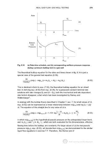
Fig. 8.14 (a) Rate-time schedule, and (b) corresponding wellbore pressure response
during a pressure buildup test in a gas well

The theoretical buildup equation for the rates and times shown in fig. 8.14 is just a
special case of the general test equation (8.39).

kh t ) m ( t ) (8.52)
−
=
i
ws
D
D
1422Q T (m(p ) m(p )) m (t + ∆ D − D ∆ D
1
1
This is identical in form to equ. (7.32), the theoretical buildup equation for an oilwell
test. In deriving equ. (8.52) from equ. (8.39), for superposed constant terminal rate
solutions with rate changes Q 1 and (0 – Q 1), both the mechanical and rate dependent
skin factors disappear, a fact which has been investigated by Ramey and
4
Wattenbarger .
In analogy with the buildup theory described in Chapter 7, sec. 7, for small values of ∆t,
equ. (8.52) can be expressed as a linear relationship between m(p ws) and log (t 1 + ∆t)/
∆t. The equation of this straight line for any value of ∆t is

kh (m(p ) m(p )) 1.151 log t +∆ t 1 ln 4t D 1 (8.53)
1
D
D
1422Q T i − ws(LIN) = t ∆ + m (t ) − 2 γ
1
1
in which m(p ws(LIN)) is the hypothetical pseudo pressure on the extrapolated linear trend,
1
and m(t ) and / 2 ln 4t /γ , which are both evaluated for the dimensionless, effective
D
D
D
1
1
flowing time before the buildup, are constants. For large values of ∆t the real pseudo
pressure m(p ws), equ. (8.52), will deviate from m(p ws(LIN)) as demonstrated for the similar
liquid flow equations in exercise 7.7. Therefore,. the Horner plot of