Page 341 - Fundamentals of Reservoir Engineering

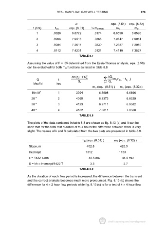
REAL GAS FLOW: GAS WELL TESTING 276

α equ. (8.51) equ. (8.32)
t (hrs) t DA equ. (8.51) ½ m D(MBH) m D m D
1 .0028 6.6772 .0174 6.6598 6.6590

2 .0056 7.0413 .0266 7.0147 7.0061
3 .0084 7.2617 .0230 7.2387 7.2080

4 .0112 7.4231 .0121 7.4110 7.3527
TABLE 8.7

Assuming the value of F = .05 determined from the Essis-Thomas analysis, equ. (8.50)
can be evaluated for both m D functions as listed in table 8.8.

−
∆ m(p) FQ n 2 n ∆ Q j
Q t Q m(t D n − t D j 1 )
D
j1 Q
−
Mscf/d hrs n = n
m D (equ. (8.51) ) m D (equ. (8.32) )
10×10 3 1 3994 6.6598 6.6596
20 " 2 4065 6.8373 6.8329
30 " 3 4123 6.9711 6.9582

40 " 4 4162 7.0811 7.0568
TABLE 8.8

The plots of the data contained in table 8.8 are shown as fig. 8.13 (a) and it can be
seen that for the total test duration of four hours the difference between them is very
slight. The values of k and S calculated from the two plots are presented in table 8.9.

m D (equ. (8.51) ) m D (equ. (8.32) )
Slope, m 402.8 426.5

Intercept 1312 1153
k = 1422 T/mh 46.6 mD 44.0 mD

S = kh × intercept/1422 T 3.3 2.7

TABLE 8.9

As the duration of each flow period is increased, the difference between the transient
and the correct analysis becomes much more pronounced. Fig. 8.13 (b) shows the
difference for 4 × 2 hour flow periods while fig. 8.13 (c) is for a test of 4 × 4 hour flow