Page 338 - Fundamentals of Reservoir Engineering

REAL GAS FLOW: GAS WELL TESTING 273

EXERCISE 8.2 SOLUTION

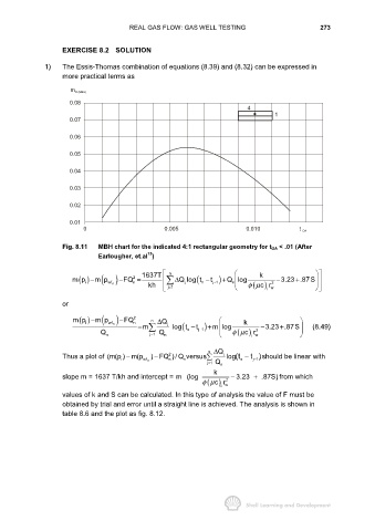
1) The Essis-Thomas combination of equations (8.39) and (8.32) can be expressed in
more practical terms as

m D (MBH)
0.08
4
1
0.07

0.06

0.05

0.04

0.03

0.02

0.01
0 0.005 0.010 t DA

Fig. 8.11 MBH chart for the indicated 4:1 rectangular geometry for t DA < .01 (After
15
Earlougher, et.al )

n
() ( )
2

m p − m p wf n − FQ = 1637T ∆ Q log t − t j 1 ) Q log φµ k i w 2 − 3.23 .87S
+
+

n
n
i
( n
j
−
kh
( ) cr

j1
=
or
() ( )
mp − mp wf n − FQ 2 n n ∆ Q j k
i
+

( n
( ) c r
Q n = m n log t − t j 1 ) m log+ φµ i w 2 − 3.23 .87S (8.49)
j1 Q
−

=
n ∆ Q
2
Thus a plot of (m(p ) m(p− wf n ) FQ )/ Q versus n j log(t − t )should be linear with
−
j 1
n
i
n
n
j1 Q
−
=
k
slope m = 1637 T/kh and intercept = m(log − 3.23 + .87S) from which
( ) cr
φµ 2
i w
values of k and S can be calculated. In this type of analysis the value of F must be
obtained by trial and error until a straight line is achieved. The analysis is shown in
table 8.6 and the plot as fig. 8.12.