Page 387 - Fundamentals of Reservoir Engineering

NATURAL WATER INFLUX 322

n1
−
∆ W j e

p = p 1− j1 (9.29)
=
n1
a − i W
ei

The values of p , the average reservoir boundary pressure, are calculated, as
n
described in section 9.3, as

p + p
−
p = n1 n (9.15)
n
2
Fetkovitch has demonstrated that using equs. (9.28) and (9.29), in a stepwise fashion,
the water influx calculated for a variety of different aquifer geometries matches closely
the results obtained using the unsteady state influx theory of Hurst and van Everdingen
for finite aquifers.

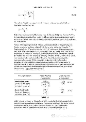
Values of the aquifer productivity index J, which depend both on the geometry and
flowing conditions, are listed in table 9.8, in Darcy units. Multiplying the radial Pl
-3
-3
functions by 7.08×10 and the linear by 1.127×10 will convert these expressions to
field units. The radial values of J for semi-steady state and steady state influx will be
recognised as identical in form to the productivity indices listed in Chapter 6, table 6.1,
for the flow of a liquid into a wellbore. The only difference is that r o, the reservoir radius,
now replaces r w, the wellbore radius. Note also that, while semi-steady state
expressions for J, equs. (9.30), are used in conjunction with the Fetkovitch
equations (9.28) and (9.29), the steady state expressions, (9.31), are used in a
different manner. In applying these values it is assumed that the water influx from the
aquifer into the reservoir is replaced by water from an external source, such as an
artesian water supply, so that the pressure

Flowing Condition Radial Aquifers Linear Aquifers
J (cc/sec/atm) J (cc/sec/atm)

Semi-steady state 2fkh 3 khw (9.30)
π
(used with drawdown r e 3 µ L
µ ln −
p
expressed as p − ) r o 4
a
Semi-steady state 2fkh khw (9.31)
π
(used with drawdown µ ln r e µ L
expressed as p − ) r o
p
i
TABLE 9.8

at the external boundary of the aquifer remains constant at its initial value p i. In this
case it is unnecessary to keep evaluating the average pressure in the aquifer since it
remains unchanged. The J values expressed in equ. (9.31) are now used in
conjunction with the drawdown measured as p i - p. Referring to equ. (9.23),