Page 391 - Fundamentals of Reservoir Engineering

NATURAL WATER INFLUX 326

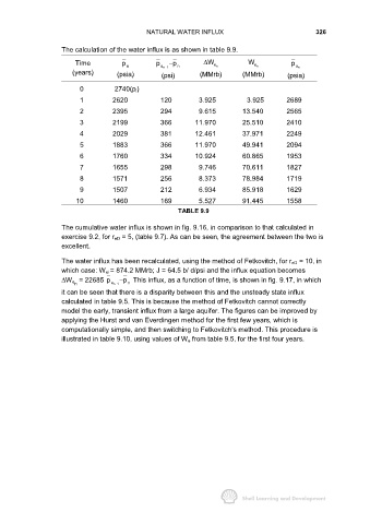
The calculation of the water influx is as shown in table 9.9.

Time p n p a n1 − p n ∆ W n e W n e p a n
−
(years) (psia) (psi) (MMrb) (MMrb) (psia)

0 2740(p i)
1 2620 120 3.925 3.925 2689

2 2395 294 9.615 13.540 2565
3 2199 366 11.970 25.510 2410
4 2029 381 12.461 37.971 2249
5 1883 366 11.970 49.941 2094

6 1760 334 10.924 60.865 1953
7 1655 298 9.746 70.611 1827
8 1571 256 8.373 78.984 1719
9 1507 212 6.934 85.918 1629

10 1460 169 5.527 91.445 1558
TABLE 9.9

The cumulative water influx is shown in fig. 9.16, in comparison to that calculated in
exercise 9.2, for r eD = 5, (table 9.7). As can be seen, the agreement between the two is
excellent.

The water influx has been recalculated, using the method of Fetkovitch, for r eD = 10, in
which case: W ei = 874.2 MMrb; J = 64.5 b/ d/psi and the influx equation becomes
∆W e = 22685 p − p This influx, as a function of time, is shown in fig. 9.17, in which
n a n1 n
−
it can be seen that there is a disparity between this and the unsteady state influx
calculated in table 9.5. This is because the method of Fetkovitch cannot correctly
model the early, transient influx from a large aquifer. The figures can be improved by
applying the Hurst and van Everdingen method for the first few years, which is
computationally simple, and then switching to Fetkovitch's method. This procedure is
illustrated in table 9.10, using values of W e from table 9.5, for the first four years.