Page 394 - Fundamentals of Reservoir Engineering

NATURAL WATER INFLUX 329

in which the cumulative gas production G p is constrained to meet a fixed market offtake
rate. The methods of Hurst and van Everdingen and Fetkovitch will be described
separately.

a) Hurst and van Everdingen

p i
pressure

p n-2
* p n-1 p n
*

T

n-2 n-1 n time

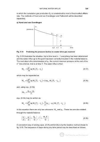
Fig. 9.18 Predicting the pressure decline in a water drive gas reservoir

Fig. 9.18 illustrates the situation. Up to time level n - 1 everything has been determined
and the water influx up to this point has been correctly included in the material balance.
The next step is the determination of p n, the current reservoir pressure at the end of the
th
n time interval, that is at time T. The water influx is then

n1
−
W = U ∆ p W T − t j D ) (9.17)
e
j
D
( D
n
j0
=
which may be expanded as
n2
−
∆
W = U ∆ p W T − t j D ) + U p W T − t D n 1 ) (9.34)
j
( D
D
D
n 1
( D
e
−
n
j0 −
=
and, using equ. (9.16)
p − p
−
∆ p n1 = n2 n
−
2
equ. (9.34) may be written as
n2 U
−
W = U ∆ p W T − t j D ) + (p n 2 − p n ) W T − t D n 1 ) (9.35)
D
( D
( D
D
j
e
−
n
j0 2 −
=
In this equation there are only two unknowns W and p . These two are also related
n e n
through the material balance
p p G W E
e
i
p
i
n
n
= 1− 1− (9.36)
Z n Z i G G
A convenient way of solving equs. (9.35) and (9.36) is by the iterative method shown in
fig. 9.19. The sequence of steps during any time period may be described as follows.