
Page 393 - Fundamentals of Reservoir Engineering
P. 393
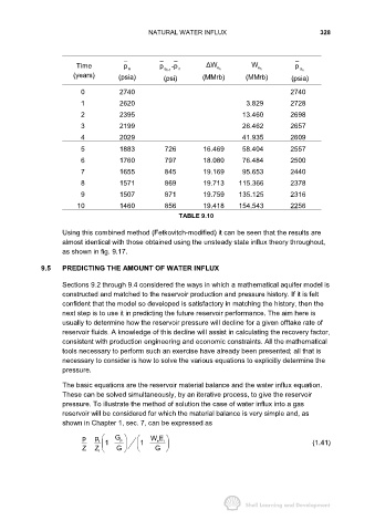
NATURAL WATER INFLUX                                   328


                         Time           p  n        p  a n-1 -p n  ∆W  n e       W  n e        p a n
                        (years)        (psia)        (psi)       (MMrb)        (MMrb)        (psia)


                           0           2740                                                  2740
                           1           2620                                    3.829         2728
                           2           2395                                   13.460         2698
                           3           2199                                   26.462         2657
                           4           2029                                   41.935         2609

                           5           1883          726         16.469       58.404         2557
                           6           1760          797         18.080       76.484         2500
                           7           1655          845         19.169       95.653         2440

                           8           1571          869         19.713      115.366         2378
                           9           1507          871         19.759      135.125         2316
                         10            1460          856         19.418      154.543         2256
                                                          TABLE 9.10

                     Using this combined method (Fetkovitch-modified) it can be seen that the results are
                     almost identical with those obtained using the unsteady state influx theory throughout,
                     as shown in fig. 9.17.

              9.5    PREDICTING THE AMOUNT OF WATER INFLUX


                     Sections 9.2 through 9.4 considered the ways in which a mathematical aquifer model is
                     constructed and matched to the reservoir production and pressure history. If it is felt
                     confident that the model so developed is satisfactory in matching the history, then the
                     next step is to use it in predicting the future reservoir performance. The aim here is
                     usually to determine how the reservoir pressure will decline for a given offtake rate of
                     reservoir fluids. A knowledge of this decline will assist in calculating the recovery factor,
                     consistent with production engineering and economic constraints. All the mathematical
                     tools necessary to perform such an exercise have already been presented; all that is
                     necessary to consider is how to solve the various equations to explicitly determine the
                     pressure.


                     The basic equations are the reservoir material balance and the water influx equation.
                     These can be solved simultaneously, by an iterative process, to give the reservoir
                     pressure. To illustrate the method of solution the case of water influx into a gas
                     reservoir will be considered for which the material balance is very simple and, as
                     shown in Chapter 1, sec. 7, can be expressed as

                           p   p      G          WE
                                       p
                                                   e
                                                     i
                                i
                             =     1−          1−                                                   (1.41)
                           Z   Z i    G           G