Page 91 - Fundamentals of Reservoir Engineering

SOME BASIC CONCEPTS IN RESERVOIR ENGINEERING 30

depletion line
p C
Z

p B
Z ab

A

G p
G

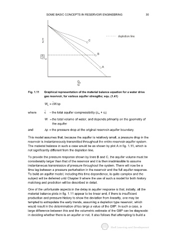
Fig. 1.11 Graphical representation of the material balance equation for a water drive
gas reservoir, for various aquifer strengths; equ. (1.41)

∆
W = cW p
e
where c = the total aquifer compressibility (c w + c f)

W = the total volume of water, and depends primarily on the geometry of
the aquifer
p
and ∆= the pressure drop at the original reservoir-aquifer boundary.

This model assumes that, because the aquifer is relatively small, a pressure drop in the
reservoir is instantaneously transmitted throughout the entire reservoir-aquifer system.
The material balance in such a case would be as shown by plot A in fig. 1.11, which is
not significantly different from the depletion line.

To provide the pressure response shown by lines B and C, the aquifer volume must be
considerably larger than that of the reservoir and it is then inadmissible to assume
instantaneous transmission of pressure throughout the system. There will now be a
time lag between a pressure perturbation in the reservoir and the full aquifer response.
To build an aquifer model, including this time dependence, is quite complex and the
subject will be deferred until Chapter 9 where the use of such a model for both history
matching and prediction will be described in detail.

One of the unfortunate aspects in the delay in aquifer response is that, initially, all the
material balance plots in fig. 1.11 appear to be linear and, if there is insufficient
production and pressure history to show the deviation from linearity, one may be
tempted to extrapolate the early trends, assuming a depletion type reservoir, which
would result in the determination of too large a value of the GIIP. In such a case, a
large difference between this and the volumetric estimate of the GIIP can be diagnostic
in deciding whether there is an aquifer or not. It also follows that attempting to build a