Page 76 - Fundamentals of The Finite Element Method for Heat and Fluid Flow

68
y
h
3 h h THE FINITE ELEMENT METHOD
3 5
4
6
z
1 2
x 1 2 z 1 2 3 z
(a) (b) (c)
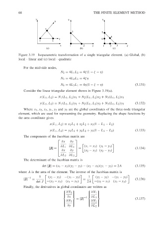
Figure 3.19 Isoparametric transformation of a single triangular element. (a) Global, (b)
local - linear and (c) local - quadratic
For the mid-side nodes,
N 2 = 4L 1 L 2 = 4ζ(1 − ζ − η)

N 4 = 4L 2 L 3 = 4ζη
N 6 = 4L 3 L 1 = 4η(1 − ζ − η) (3.131)
Consider the linear triangular element shown in Figure 3.19(a).

x(L 1 ,L 2 ) = N 1 (L 1 ,L 2 )x 1 + N 2 (L 1 ,L 2 )x 2 + N 3 (L 1 ,L 2 )x 3
y(L 1 ,L 2 ) = N 1 (L 1 ,L 2 )y 1 + N 2 (L 1 ,L 2 )y 2 + N 3 (L 1 ,L 2 )y 3 (3.132)
Where x 1 ,x 2 ,x 3 ,y 1 ,y 2 and y 3 are the global coordinates of the three-node triangular
element, which are used for representing the geometry. Replacing the shape functions by
the area coordinate gives
x(L 1 ,L 2 ) = x 1 L 1 + x 2 L 2 + x 3 (1 − L 1 − L 2 )

y(L 1 ,L 2 ) = y 1 L 1 + y 2 L 2 + y 3 (1 − L 1 − L 2 ) (3.133)
The components of the Jacobian matrix are
∂x ∂y
 
(x 1 − x 3 )(y 1 − y 3 )

 
[J] =  ∂L 1 ∂L 1  = (3.134)
 ∂x
∂y  (x 2 − x 3 )(y 2 − y 3 )
∂L 2 ∂L 2
The determinant of the Jacobian matrix is
det [J] = (x 1 − x 3 )(y 2 − y 3 ) − (x 2 − x 3 )(y 1 − y 3 ) = 2A (3.135)
where A is the area of the element. The inverse of the Jacobian matrix is

1 (y 2 − y 3 ) −(y 1 − y 3 ) 1 (y 2 − y 3 ) −(y 1 − y 3 )
−1
[J] = = (3.136)
det J −(x 2 − x 3 )(x 1 − x 3 ) 2A −(x 2 − x 3 )(x 1 − x 3 )
Finally, the derivatives in global coordinates are written as
   
 ∂N 1   ∂N 1 
   
∂x −1 ∂L 1
   
= [J] (3.137)
 ∂N 1  ∂N 1 
   
∂y ∂L 2
   