Page 73 - Fundamentals of The Finite Element Method for Heat and Fluid Flow

THE FINITE ELEMENT METHOD
Therefore, we can write



 ∂N i   ∂N i  65

   
∂x −1 ∂ζ
   
= [J] (3.115)
 ∂N i   ∂N i 
   
   
∂y ∂η
Note that the inverse of the Jacobian matrix [J] −1 is calculated as
∂y ∂y
 
−
1  ∂η ∂ζ 
−1
[J] =   (3.116)
det [J]  ∂x ∂x 
−
∂η ∂ζ
The derivatives have to be numerically evaluated at each integration point, as a closed-
form solution does not exist
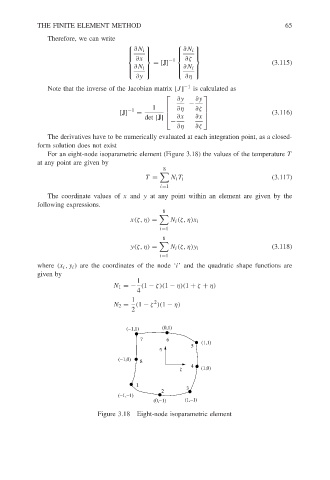
For an eight-node isoparametric element (Figure 3.18) the values of the temperature T
at any point are given by
8

T = N i T i (3.117)
i=1
The coordinate values of x and y at any point within an element are given by the
following expressions.
8

x(ζ, η) = N i (ζ, η)x i
i=1
8

y(ζ, η) = N i (ζ, η)y i (3.118)
i=1
where (x i ,y i ) are the coordinates of the node ‘i’ and the quadratic shape functions are
given by
1
N 1 =− (1 − ζ)(1 − η)(1 + ζ + η)
4
1 2
N 2 = (1 − ζ )(1 − η)
2
(−1,1) (0,1)
7 6
(1,1)
5
h
(−1,0)
8
4
(1,0)
z
1
3
2
(−1,−1)
(0,−1) (1,−1)
Figure 3.18 Eight-node isoparametric element