Page 68 - Fundamentals of The Finite Element Method for Heat and Fluid Flow

60
The gradient matrix can be written as

∂T  THE FINITE ELEMENT METHOD
 
  T 1
   
∂x 1 −(a − y) (a − y) (a + y) −(a + y) T 2
   
{g}= =
4ab −(b − x) −(b + x) (b + x) (b − x)
 ∂T  T 3
   
∂y T 4
   
= [B]{T} (3.96)
The [B] matrix is written as

1 −(1 − η) (1 − η) (1 + η) −(1 + η)
[B] = (3.97)
4 −(1 − ζ) −(1 + ζ) (1 + ζ) (1 − ζ)
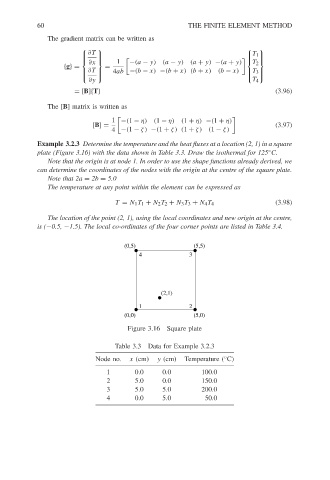
Example 3.2.3 Determine the temperature and the heat fluxes at a location (2, 1) in a square
◦
plate (Figure 3.16) with the data shown in Table 3.3. Draw the isothermal for 125 C.
Note that the origin is at node 1. In order to use the shape functions already derived, we
can determine the coordinates of the nodes with the origin at the centre of the square plate.
Note that 2a = 2b = 5.0
The temperature at any point within the element can be expressed as
T = N 1 T 1 + N 2 T 2 + N 3 T 3 + N 4 T 4 (3.98)
The location of the point (2, 1), using the local coordinates and new origin at the centre,
is (−0.5, −1.5). The local co-ordinates of the four corner points are listed in Table 3.4.

(0,5) (5,5)
4 3

(2,1)

1 2
(0,0) (5,0)

Figure 3.16 Square plate

Table 3.3 Data for Example 3.2.3
Node no. x (cm) y (cm) Temperature ( C)
◦
1 0.0 0.0 100.0
2 5.0 0.0 150.0
3 5.0 5.0 200.0
4 0.0 5.0 50.0