Page 66 - Fundamentals of The Finite Element Method for Heat and Fluid Flow

58
(x 3 ,y 3 )
y
3 THE FINITE ELEMENT METHOD
(x 4 ,y 4 )
4
1 2
(x 2 ,y 2 )
(x 1 ,y 1 )
x
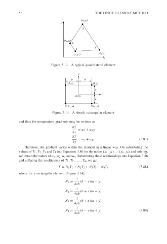
Figure 3.13 A typical quadrilateral element

y
b b
4 (−b,a) 3 (b,a)
a
x
(0,0)
a
1(−b,−a) 2(b,−a)
Figure 3.14 A simple rectangular element

and thus the temperature gradients may be written as
∂T
= α 2 + α 4 y
∂x
∂T
= α 3 + α 4 x (3.87)
∂y
Therefore, the gradient varies within the element in a linear way. On substituting the
values of T 1 ,T 2 ,T 3 and T 4 into Equation 3.86 for the nodes (x 1 ,y 1 )... (x 4 ,y 4 ) and solving,
we obtain the values of α 1 ,α 2 ,α 3 and α 4 . Substituting these relationships into Equation 3.86
and collating the coefficients of T 1 ,T 2 ,... ,T 4 ,weget

T = N 1 T 1 + N 2 T 2 + N 3 T 3 + N 4 T 4 (3.88)
where for a rectangular element (Figure 3.14),
1
N 1 = (b − x)(a − y)
4ab
1
N 2 = (b + x)(a − y)
4ab
1
N 3 = (b + x)(a + y)
4ab
1
N 4 = (b − x)(a + y) (3.89)
4ab