Page 62 - Fundamentals of The Finite Element Method for Heat and Fluid Flow

54
and
(3.62)
L k = y THE FINITE ELEMENT METHOD
2.5
From Equation 3.55, we get
x y
L i = 1 − − (3.63)
4 2.5
At (x, y) = (2, 1),wehave
L i = 0.1 = N i
L j = 0.5 = N j

L k = 0.4 = N k (3.64)
Note that these local coordinates are exactly the same as the shape function values
calculated in Example 3.2.2

3.2.5 Quadratic triangular elements

We can write a quadratic approximation over a triangular element as
2
2
T = α 1 + α 2 x + α 3 y + α 4 x + α 5 y + α 6 xy (3.65)
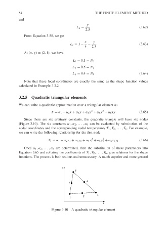
Since there are six arbitrary constants, the quadratic triangle will have six nodes
(Figure 3.10). The six constants α 1 ,α 2 ,... ,α 6 can be evaluated by substitution of the
nodal coordinates and the corresponding nodal temperatures T 1 ,T 2 ,... ,T 6 . For example,
we can write the following relationship for the first node:

2 2
T 1 = α 1 + α 2 x 1 + α 3 y 1 + α 4 x + α 5 y + α 6 x 1 y 1 (3.66)
1 1
Once α 1 ,α 2 ,... ,α 6 are determined, then the substitution of these parameters into
Equation 3.65 and collating the coefficients of T 1 ,T 2 ,... ,T 6 , give relations for the shape
functions. The process is both tedious and unnecessary. A much superior and more general

y
5

4
6

3
2
1
x
Figure 3.10 A quadratic triangular element