Page 67 - Fundamentals of The Finite Element Method for Heat and Fluid Flow

THE FINITE ELEMENT METHOD
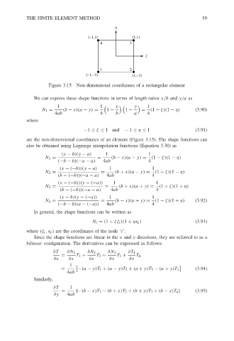
(−1,1) h (1,1) 59
4 3
z

1 2
(−1,−1) (1,−1)

Figure 3.15 Non-dimensional coordinates of a rectangular element

We can express these shape functions in terms of length ratios x/b and y/a as
1 1 x y 1
N 1 = (b − x)(a − y) = 1 − 1 − = (1 − ζ)(1 − η) (3.90)
4ab 4 b a 4
where
−1 ≤ ζ ≤ 1and − 1 ≤ η ≤ 1 (3.91)

are the non-dimensional coordinates of an element (Figure 3.15). The shape functions can
also be obtained using Lagrange interpolation functions (Equation 3.30) as
(x − b)(y − a) 1 1
N 1 = = (b − x)(a − y) = (1 − ζ)(1 − η)
(−b − b)(−a − a) 4ab 4
(x − (−b))(y − a) 1 1
N 2 = = (b + x)(a − y) = (1 + ζ)(1 − η)
(b − (−b))(−a − a) 4ab 4
(x − (−b))(y − (−a)) 1 1
N 3 = = (b + x)(a + y) = (1 + ζ)(1 + η)
(b − (−b))(−a − a) 4ab 4
(x − b)(y − (−a)) 1 1
N 4 = = (b − x)(a + y) = (1 − ζ)(1 + η) (3.92)
(−b − b)(a − (−a)) 4ab 4
In general, the shape functions can be written as
N i = (1 + ζζ i )(1 + ηη i ) (3.93)

where (ζ i ,η i ) are the coordinates of the node ‘i’.
Since the shape functions are linear in the x and y directions, they are referred to as a
bilinear configuration. The derivatives can be expressed as follows:
∂T ∂N 1 ∂N 2 ∂N 3 ∂T 4
= T 1 + T 2 + T 3 + T 4
∂x ∂x ∂x ∂x ∂x
1
= −(a − y)T 1 + (a − y)T 2 + (a + y)T 3 − (a + y)T 4 (3.94)
4ab
Similarly,
∂T 1
= [−(b − x)T 1 − (b + x)T 2 + (b + x)T 3 + (b − x)T 4 ] (3.95)
∂y 4ab