Page 69 - Fundamentals of The Finite Element Method for Heat and Fluid Flow

THE FINITE ELEMENT METHOD
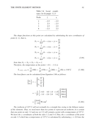
Table 3.4 Local
nates for Example 3.2.3
η
Node ζ coordi- 61
1 −2.5 −2.5
2 2.5 −2.5
3 2.5 2.5
4 −2.5 2.5

The shape functions at this point are calculated by substituting the new coordinates of
point (2, 1), that is,
1 12
N 1 = (b − x)(a − y) =
4ab 25
1 8
N 2 = (b + x)(a − y) =
4ab 25
1 2
N 3 = (b − x)(a + y) =
4ab 25
1 3
N 4 = (b − x)(a + y) = (3.99)
4ab 25
Note that N 1 + N 2 + N 3 + N 4 = 1.
Therefore, the temperature at the point (−0.5, −1.5) is
12 8 2 3
◦
T (−0.5,−1.5) = (100) + (150) + (200) + (50) = 118 C (3.100)
25 25 25 25
The heat fluxes can be calculated from Equation 3.96 as follows:
 
∂T
 
 k x

 
q x ∂x
=−
q y  ∂T 
k y 


∂y
 
100.0
2 −4.0 4.01.0 −1.0  150.0 



=−
25 −3.0 −2.02.0 3.0 200.0
 
50.0
 

28.0 2
= W/cm (3.101)
4.0
◦
The isotherm of 125 C will not normally be a straight line owing to the bilinear nature
of the elements. Thus, we need more than two points to represent an isotherm. It is certain
◦
that one point on side 1-2 and one on 3-4 will contain a point with a temperature of 125 C.
We know the y coordinates of both the sides 1-2 and 3-4. Thus, the x coordinate of the point
◦
on side 1-2 which has a temperature of 125 C is calculated by substituting y = 0.0 into the