Page 70 - Fundamentals of The Finite Element Method for Heat and Fluid Flow

THE FINITE ELEMENT METHOD
62
temperature distribution of Equation 3.98, that is,
125.0 = 1 [(2.5 − x)(2.5 − 0.0)100.0 + (2.5 + x)(2.5 − 0.0)150
25
+(2.5 + x)(2.5 + 0.0)200.0 + (2.5 − x)(2.5 + 0.0)50.0] (3.102)
which gives x = 2.5 and similarly, if we substitute a value of y = 5.0 for the side 3-4 the
result is x = 2.5. These coordinates can be written in a local form as (0.0, −2.5) and (0.0,
2.5). From the two points found, it is clear that the 125 C isotherm crosses all horizontal
◦
lines between the bottom and top sides. Therefore, to determine another point, we can assume
a‘y’ value of 2.5 (0.0, in local form) and on substituting into Equation 3.98 results in an x
coordinate of 2.5 (0.0, in local form). Connecting all three points will generate the 125 C
◦
isotherm.

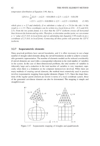
3.2.7 Isoparametric elements

Many practical problems have curved boundaries, and it is often necessary to use a large
number of straight-sided elements along the curved boundaries in order to achieve a reason-
able geometric representation. The number of elements needed can be reduced considerably
if curved elements are used with a consequential reduction in the total number of variables
in the system. In the case of three-dimensional problems, the total number of variables is
inherently large and a reduction in the total number of variables is very important, espe-
cially when there is a limitation on the computer memory/cost involved. While there are
many methods of creating curved elements, the method most extensively used in practice
involves isoparametric mapping from regular elements (Figure 3.17). Since the shape func-
tions of the regular parent element are known in terms of a local coordinate system, those
of the generated curvilinear element can also be determined. The mapping is simple and
straightforward.

y

L 2 = 0
L 1 = 0 = 0
L = 0 L 1
2

L = 0
3
= 0
L 3
(−1,1) h (1,1)
h

z z

x
(−1,−1) (1,−1)
Figure 3.17 Isoparametric mapping of triangles and quadrilaterals