Page 358 - Fundamentals of Water Treatment Unit Processes : Physical, Chemical, and Biological

Flocculation 313

11.5.3 PLANT DESIGN
While unit processes are the foci of any plant design, a host of
other considerations are necessary to support any process
functioning. The layout of the overall plan showing all unit
processes as they are integrated as a system is the first task.
Other tasks required include the sizing of pipes, motors,
meters, etc.; selection of materials for pipes, paddle wheels,
walls; locations of pipes and valves; and methods of adjust-
ment for paddle-wheel rotational velocity. How all of this
fits together is shown in drawings with specifications giving
supplemental details. A modern adjunct to traditional draw-
ings is an animation derived from the drawings by means of
software.
Figure CD11.17a and b are excerpts from ‘‘walk-through’’
animations illustrating the design for the Floc-Sed basin 2000
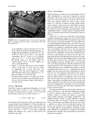
FIGURE 11.14 Flocculation basin for 76 L=min (20 gpm) pilot addition to the Fort Collins WTP. The animation starts with a
plant at Engineering Research Center, Colorado State University, view seen upon entering the building. The plant addition has
Fort Collins, CO. two identical parallel treatment trains, each with a four-com-
partment flocculation basin; the flow leaves the fourth basin
and then to an assembly of Lamella plate settlers on the east
given in Rushton’s work (see Section 10.3.3.3). The side of the building. The first view is from the northwest
power number is affected by Reynolds number as a corner looking south along the west side of the building and
5
straight-line relationship in the range, R < 10 , and along the first compartments of both trains. Walking south, a
1
5
for R > 10 , P 4.1. If G 100 s , as in the first left turn is made heading east between the two trains. The
5
compartment, R 10 , which is in the turbulent plate settler basins are encountered at the end of the floc basin.
1
range. If G 15 s , as in the third compartment, Walking to the east side of the building and then south along
R 20,000, which is in the laminar range and the plate settler basin, the tops of the plates are seen to the
Camp’s equation (10.5) G ¼ [P=mV] 0.5 applies, i.e., right. Walking around the assembly gives a more detailed
with m in the denominator. view of the third compartment of the flocculation basin. The
. Figure 11.15d shows shaft power versus rotational serpentine path from one compartment to another is clearly
velocity of the shaft. As seen, the curve shows visible at this point. Also, the detail of the number of arms for
an exponential rise in power with rpm with each paddle wheel may be seen, i.e., compartments #1 and #2
exponent ¼ 2.26. The power required for a given paddles each have three arms while compartments #3 and #4
shaft rotational velocity can be obtained. For n ¼ 12 each have two. The separation walls between each compart-
rpm, for example, P 10 W (0.013 hp). ment are only to channel the water flow and are made of
. The plots shown in Figure 11.15 apply only for the redwood. Figure CD11.17b (animation) starts at the same
system tested. The nature of the relationships shown, place but the walk leads down the stairs to the lower level
however, and their general shapes should apply to where a pipe gallery and paddle-wheel motors are seen; the
any other system. motors are larger in size as the walk moves from compartment
#4 toward compartment #1. Turning the corner, the main pipe
11.5.2.3 Slip Factor gallery is seen with large pipes that deliver coagulated water
to each of the floc basins.
Table CD11.8 shows the application of Equation 11.19 to the
As stated previously, design walk-through animations are
data of Table CD11.7 to give k, i.e., the ‘‘slip factor,’’ values
software derivatives of the traditional engineering drawings
for different rotational velocities. Figure 11.16 is a plot of the
as done by drawing software (such as AutoCade). They
data showing k versus rpm as a linear relation, i.e.,
provide a means to visualize the project as constructed,
which permits inspection and perhaps modifications. The
k ¼ 0:074 þ 0:007 rpm (11:27)
animation permits ‘‘seeing’’ in places difficult to visualize
by drawings alone. For example, at about 0.45 completion
The intercept (0.074) and slope (0.007) may differ from one of (b), a recessed space with sludge drain pipes is seen, which
system to another, but the Equation 11.27 form should be true is difficult to visualize from the traditional drawings. The
regardless of the system (such as model or full scale). If a slip pseudo walk through lets the designer determine whether,
factor is selected for a design that lacks empirical data, then for example, pipes are crossing paths of one another at some
Camp’s slip factor, i.e., 0.24 < k < 0.32 gives a reasonable point, whether the overall layout is reasonable, and whether
estimate; for reference, the k values in Table CD11.8 are the plant seems operable. These same points are of interest to
within the same range. the persons in operation.