Page 355 - Fundamentals of Water Treatment Unit Processes : Physical, Chemical, and Biological

310 Fundamentals of Water Treatment Unit Processes: Physical, Chemical, and Biological

1
8 design shown (diameter ¼ 3.9 m (12.8 ft) and G ¼ 60 s )is
10 1.323 kW (1.8 hp). Using a motor efficiency of 0.67, the
7
motor power would be 1.97 kW (2.6 hp), which corresponds
to similar installations in practice (albeit the diameter used
6 Motor capacity 8
in this example is larger than used in most installations in
practice).
5
Power (kW) 4 6 Power (hp) 11.5.2 MODEL FLOCCULATION BASIN

3 Power to shaft 4 Figure 11.14 shows a flocculation basin with three compart-
ments with paddle wheels, each with vertical shaft. The motor
2
for the first compartment was mounted on a bearing plate
Friction losses 2
with lever arm attached to the motor frame and with a force
1
gage attached at the end of the lever arm. This arrangement
permitted measurement of the force exerted by the lever arm
0 0
500 1000 1500 2000 2500 3000 and calculation of torque. The rotational velocity for a given
motor controller setting could be measured simply by count-
Shaft speed (rpm)
ing the rotations with a stopwatch.
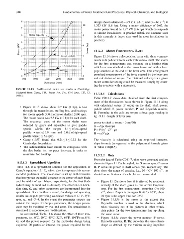
FIGURE 11.13 Paddle-wheel motor test results at Cambridge.
(Adapted from Camp, T.R., Trans. Am. Soc. Civil Eng., 120, 13, 11.5.2.1 Calculations
1955.)
Table CD11.7 shows data obtained from the first compart-
ment of the flocculation basin shown in Figure 11.14 along
with calculated values of torque on the shaft, shaft power,
. Figure 11.13 shows about 0.7 kW (1 hp), is lost
paddle wheel G, power number, P, and Reynolds number,
through the transmission, stuffing box, and bearings
R. Formulae in the cells are torque ¼ force gage reading in
for motor speeds 500 n(motor shaft) 2600 rpm.
kg 9.81 length of lever arm
The motor power was 7.5 kW (10 hp) for each shaft.
The rotational speed of the motor shafts were power to shaft ¼ torque (rpm=60)
reduced by gears and adjustable to give paddle G ¼ P=mV(comp)
speeds within the ranges 1.1 n(low-speed P ¼ P=(n D r)
5
3
paddle wheel) 2.9 rpm and 2.0 n(high-speed R ¼ vD r=m
2
paddle wheel) 5.2 rpm.
. Camp (1955) found that 0.24 k 0.32 for the The viscosity is calculated using an empirical intercept-
Cambridge flocculators. slope formula (as opposed to the polynomial formula given
. The sedimentation basin should be contiguous with in Table CDQR.5).
the floc basin, i.e., no pipes between, in order to
minimize floc breakup.
11.5.2.2 Plots
From the data of Table CD11.7, plots were generated and are
11.5.1.3 Spreadsheet Algorithm shown in Figure 11.15a through d, for G versus rpm, G versus
Table 11.6 is a spreadsheet solution for the application of R, P versus R, power-to-shaft versus rpm, respectively. The
1
Camp’s equation (11.19), which also incorporates his recom- plots show the range of practice, i.e., 10 G 100 s ,as
mended guidelines. The spreadsheet is set up with formulae shaded areas. Features of each plot are enumerated.
that incorporate the radial distance to the center of each blade
and the width of each blade, respectively, for the first blade . Figure 11.15a shows how G is affected by rotational
(which may be modified as desired). The criterion for deten- velocity of the shaft, given as rpm at two temperat-
tion time, G, and other parameters are incorporated into the ures. For the first compartment assuming G 100
1
spreadsheet. Once the flow is stated, the design and operating s , about 13 rpm is the upper limit for 108C; about
results are outputs providing calculated values of G, P, P=V, 10 rpm is the upper limit for 228C.
rpm, v b , and G u. In the event the parameter outputs are . Figure 11.15b is the same as (a) except that
outside the ranges of Camp’s guidelines, the design param- Reynolds number is used as the abscissa, which
eters may be modified by trial and error. The spreadsheet is takes viscosity out of the picture; in other words,
structured to accommodate modifications. data points for the two temperatures line up along
As constructed, Table 11.6 shows the effect of three tem- the same curve.
peratures, i.e., 08C, 208C, 408C (328F, 688F, 1048F) on P=V, . Figure 11.15c shows the power number, P versus
G, and the power required for the particular design being Reynolds number, R. The curve has the same classic
explored. Of particular interest, the power required for the shape as defined by the various mixing impellers