Page 711 - Fundamentals of Water Treatment Unit Processes : Physical, Chemical, and Biological

666 Fundamentals of Water Treatment Unit Processes: Physical, Chemical, and Biological

pH TABLE CD21.2
0 1 2 3 4 5 6 7 8 9 10 11 12 13 14 2þ
0 Concentrations of [Ca ] as a Function of pH
2+
[Ca ]= 0.1 mol/L a
1 C ¼ 0.01 mol=L
–
2+
2 p[Ca ]+ 2p[OH ]=5.3 K a ¼ 5.01E 06
pK a ¼ 5.3
3
p [H ] p log [OH ]

þ
4
pH [H ] (mol=L) [OH ] [OH ] (mol=L) p[Ca ]
2þ

þ
5
Precipitation zone 0.00 0.00 1.00Eþ00 14 14 1.00E 14 22.7000
6 1.00 1.00 1.00E 01 13 13 1.00E 13 20.7000
p[Ca 2+ ] 7 2.00 2.00 1.00E 02 12 12 1.00E 12 18.7000
8 3.00 3.00 1.00E 03 11 11 1.00E 11 16.7000
4.00 4.00 1.00E 04 10 10 1.00E 10 14.7000
9 5.00 5.00 1.00E 05 9 9 1.00E 09 12.7000
p[OH] pH
10 6.00 6.00 1.00E 06 8 8 1.00E 08 10.7000
7.00 7.00 1.00E 07 7 7 1.00E 07 8.7000
11
8.00 8.00 1.00E 08 6 6 1.00E 06 6.7000
12
9.00 9.00 1.00E 09 5 5 1.00E 05 4.7000
13 10.00 10.00 1.00E 10 4 4 1.00E 04 2.7000
14 11.00 11.00 1.00E 11 3 3 1.00E 03 0.7000
11.20 11.20 6.31E 12 2.8 2.8 1.58E 03 0.3000
FIGURE CD21.1 pC versus pH diagram for Ca . 11.30 11.30 5.01E 12 2.7 2.7 2.00E 03 0.1000
2þ
11.40 11.40 3.98E 12 2.6 2.6 2.51E 03 0.1000
11.60 11.60 2.51E 12 2.4 2.4 3.98E 03 0.5000
Discussion
11.80 11.80 1.58E 12 2.2 2.2 6.31E 03 0.9000
Figure CD21.1 (see also Figure 6-3, p. 255, Snoeyink and
Jenkins) shows graphically the coordinate point where the 12.00 12.00 1.00E 12 2 2 1.00E 02 1.3000
13.00 13.00 1.00E 13 1 1 1.00E 01 3.3000
solution occurs, that is, (pH, pC) ¼ (pH ¼ 11.85, C ¼ 0.1
mol Ca =L). As seen, Example ‘‘Express (5) in log form’’ 14.00 14.00 1.00E 14 0 0 1.00Eþ00 5.3000
2þ
second equation, that is, p[Ca ] þ 2p[OH ] ¼ 5.3,
2þ

expresses the equilibrium relation seen as the line passing
through the point ‘‘a,’’ the system point. The solution is 22
‘‘supersaturated’’ in the zone to the right of the equilibrium 20
line. The area to the left represents undersaturation. In 18 1
other words, precipitation may be induced by imposing 16 Fe 3+
high pH conditions; the lower the Ca 2þ concentration, that 14 FeOH 2+ O 2
is, as p[Ca ] increases, the higher the pH required to 12 H O
2þ
cause precipitation. Table CD21.2 was the set up used 10 2
for the calculations; Figure CD21.1 is linked to Table 8 0.5
CD21.2 (using the spreadsheet). Table CD21.2 may be pε 6 Fe(OH) (s) E (volts)
used as a template for other precipitates as well (modified 4 2+ 3
to fit the chemical equations). 2 Fe
0 0
21.2.1.5 p«–pH Diagrams –2
–4 H O
2
For reactions in which both electron transfer and proton H
–6 2
transfer occur, both control the species present at any given –8 FeOH + –0.5
(pH, pe) coordinate. By plotting the equilibrium relations –10 Fe(OH) (s)
2
between different species in terms of pH and pe, the bound- –12
0 1 2 3 4 5 6 7 8 9 1011121314
aries between species can be delineated (see Snoeyink and
pH
Jenkins, 1980, pp. 358–363). Figure 21.2 shows such a plot
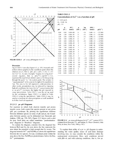
for iron. Such plots are called sometimes ‘‘predominance- FIGURE 21.2 pe versus pH diagram for Fe –Fe 2þ system (258C).
2þ
area’’ diagrams or ‘‘Pourbaix’’ diagrams. (Adapted from Snoeyink, V.L. and Jenkins, D., Water Chemistry,John
To explain the diagram, consider first, the diagonal line Wiley & Sons, New York, 1980, p. 362.)
between H 2 O and O 2 ; the area above the line represents the
area where the potential is high enough that O 2 occurs. The To explain their utility of a pe vs. pH diagram in under-
diagonal between Fe 2þ and Fe(OH) 3 (s) shows the equilibrium standing the water quality issues of acid–mine drainage
between the two species. For any coordinate point within the involving iron, we may consider the conditions within the
area above the line, Fe(OH) 3 (s) predominates; below the line, underground environment. Here, acid conditions prevail
Fe 2þ predominates. with pH 4, and with reducing conditions, that is, low pe.