Page 742 - Fundamentals of Water Treatment Unit Processes : Physical, Chemical, and Biological

Biological Reactions and Kinetics 697

0.2 The Arrhenius equation is also given in the form,
–1
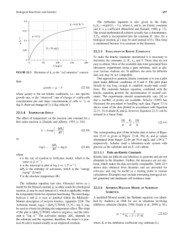
ˆ μ =0.21 (h )
k 2 =k 1 ¼ exp(K(T 2 T 1 ), where k 1 and k 2 are kinetic constants
and K is a coefficient (Benefield and Randall, 1980, p. 12).
0.15
The actual mathematical solution actually has a denominator,
μ= 0.5 μ ˆ T 1 T 2 , which is incorporated into the constant, K. Also, for a
μ (h –1 ) 0.1 biological reaction, bm’s may be used instead of k’s. This form
is mentioned because it is common in the literature.
K =50 mg/L
s
0.05
22.5.5 EVALUATION OF KINETIC CONSTANTS
To make the kinetic equations operational it is necessary to
0 determine the constants, bm, K s , k d , and Y. These data are not
0 50 100 150 200
easy to obtain. Most of the available data were generated from
S (mg/L)
laboratory experiments using a pure substrate, such as glu-
cose, lactose, maltose, etc. In addition, the units for different
FIGURE 22.3 Illustration of K s as the ‘‘half-saturation’’ constant.
data sets may be not compatible.
One approach to generate kinetic constants is to run a pilot
then plant under different conditions of X and S. The pilot plant
should be run long enough to establish steady-state condi-
m(net) ¼ m b (22:38)
tions. The materials balance equation, combined with the
kinetic equation, permits the determination of needed con-
where m(net) is the net kinetic coefficient, i.e., net specific
stants. The experiments should systematically vary [S] so
growth rate, or the ‘‘observed’’ rate of change of viable-cells
1
concentration per unit mass concentration of cells (s ); or that a number of points are available. Schulze (1965) has
3 3 illustrated the procedure in handling such data. Figure 22.4a
(kg X observed change=m =s=)=(kg cells=m ).
shows some of his data plotted in accordance with Equation
22.31. To evaluate K s and bm, however, Equation 22.31 can be
22.5.4 TEMPERATURE EFFECT
restated in a linear form:
The effect of temperature on the reaction rate constant for a
[S] K s [S]
first-order reaction is (Daniels and Alberty, 1955, p. 341) (22:41)
m
m
m ¼ _ þ _

DH a
(22:39)
RT The corresponding plot of the Schulze data in terms of Equa-
k ¼ A exp
tion 22.41 is given as Figure 22.4b. The K s and bm values
or determined from Figure 22.4b are 95.4 mg=L and 1.09 h 1
respectively. Schulze used a laboratory-scale system with
DH a
þ log A (22:40) glucose as the substrate and an E. coli culture.
log k ¼
RT
22.5.5.1 Data on Kinetic Constants
where
Kinetic data are difficult and laborious to generate and are not
k is the rate of reaction in Arrhenius model, which is the
1 abundant in the literature. Further, the measures are not uni-
same as bm (s )
1 form, which makes the data not easily comparable. Table 22.9
A is the intercept in plot of log k vs. 1=T (s )
shows data obtained from literature and are provided for
DH a is the enthalpy of activation, which is the ‘‘energy
reference and may be useful as a starting point in various
hump’’ (J=mol)
calculations. Examples may include estimating biological sol-
T is the absolute temperature (K)
ids generated and minimum cell residence time.
The Arrhenius equation (see also, Glossary) serves as a
model for the Monod constant, bm; in other words for a biological 22.5.6 ANDREWS=HALDANE MODEL OF SUBSTRATE
reaction, bm may beusedinstead of k, which is applicable within
INHIBITION
the temperature limits for organism functioning. The interchange
between k and bm is seen as justified within the Michaelis– A modified Monod model, the Haldane equation was identi-
Menten description of enzyme kinetics, Appendix 22.B. The fied by Andrews in 1968 for use in situations involving
Arrhenius model, log bm ¼ [DH a =2=303R] [1=T] þ log A, may inhibitory substrate (Suidan, 1988; Grady et al., 1999, p. 81),
be used as a basis for plotting the temperature effect. The slope
of the plot is [DH a =2=303R], which is negative, and the inter- _ S
m ¼ m (22:42)
2
cept is ‘‘log A.’’ The activation energy, DH a , depends on K s þ S þ S =K i
the substrate and the organism; therefore, the slope is a prac-
tical fit and is treated usually as an empirical constant. where K i is the inhibition coefficient (mg substrate=L).