Page 120 - Geometric Modeling and Algebraic Geometry

7 Curve Parametrization Exploiting the Newton Polygon 121
v
v
planes, which are open subsets, depending on whether ¯u¯ =0, ¯x¯ =0, ¯x¯ =0 or
y
y
¯ u¯ =0. Again we introduce local coordinates:
⎧ ¯ x y
⎪ (1, 1, , )=:(1, 1,u 1 ,v 1 ) if ¯u¯v =0
¯
¯ u v
⎨ u ¯ ¯ ¯ y
⎪
( , 1, 1, )=:(v 2 , 1, 1,u 2 ) if ¯x¯v =0
y
(¯u, ¯v, ¯x, ¯)= ¯ x ¯ u v ¯ v
⎪ ( , , 1, 1) =: (u 3 ,v 3 , 1, 1) if ¯x¯y =0
¯
⎪ x y
(1, , , 1) =: (1,u 4 ,v 4 , 1) if ¯u¯y =0
⎩ ¯ ¯ v ¯ ¯ x
¯ y ¯ u
Now changing from one coordinate system to the other we find
v i = u −1
i−1 ,u i = v i−1
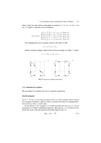
and the coordinate change could be derived from a rectangle (see figure 7.1 right):
v i =(−u i−1 ), u i = v i−1
Z 2 u 4 v 4 u 3 v 3 Z 2

v 3
u 3

u 2
v 1
v 1
u 1
u 1
v 2
Fig. 7.1. Isosceles triangles and squares v 2 u 2

7.2.3 Smooth toric surfaces
The preceding two examples give rise to a general construction.

Smooth polygons

Let Π ⊂ R be a convex lattice polygon, that is a convex polygon whose vertices
2
have integral coordinates. Label its vertices cyclically and attach two minimal direc-
tion vectors u i and v i to each vertex.
To proceed as in the examples, we would need that each pair (u i , v i ) can be
expressed as a Z-linear combination using any other pair (u j , v j ). For this it is suf-
ficient that each of the pairs generates the entire integer lattice, i.e.

Zu i + Zv i = Z . (7.2)
2