Page 119 - Geometric Modeling and Algebraic Geometry

120 T. Beck and J. Schicho
tried to make the explanation of the necessary concepts and the description of the
algorithm as self-contained as possible.
Once and for all let K denote a perfect field, the field of definition, and K an alge-
braic closure of K. Further let f ∈ K[x, y] be an absolutely irreducible polynomial,
i.e. irreducible in K[x, y].

7.2 Toric geometry

In this section we introduce just as much of toric geometry as we need in this paper. A
good general introduction to toric geometry is [3]. We focus on the fact that smooth
toric surfaces are generalizations of the standard surfaces P and P × P .
1
1
2
K K K
7.2.1 The projective plane P 2
K
v
y
The projective plane is the set of points (¯ :¯x :¯) subject to the equivalence relation
v
v
y
y
(¯ :¯x :¯)=(λ¯ : λ¯x : λ¯) for λ =0. It can be covered by 3 affine planes, which
are open subsets, depending on whether ¯ =0, ¯x =0 or ¯ =0. We can introduce
y
v
local coordinates on each of these open subsets:
⎧ ¯ x ¯ y
v
⎨ (1 : ¯ v : )=:(1 : u 1 : v 1 ) if ¯ =0
¯ v
¯ y
¯ v
v
y
(¯ :¯x :¯)= ( :1: )=:(v 2 :1: u 2 ) if ¯x =0
¯ x
¯ x
⎩ v ¯ x
( : :1) =: (u 3 : v 3 :1) if ¯ =0
y
¯
¯ y ¯ y
If both sides are defined, i.e. on the intersection of open subsets, we see that
v i = u −1 ,u i = v i−1 u −1 . (7.1)
i−1 i−1
Here we assumed for convenience that indices are cyclically arranged, i.e. u 3 = u 0
and v 3 = v 0 .
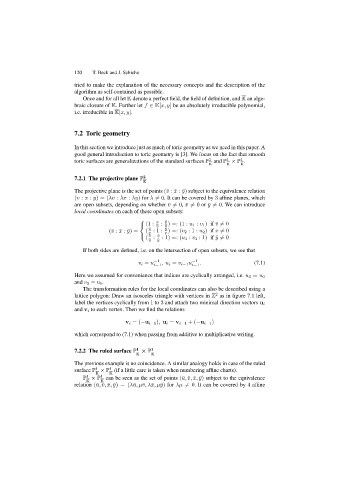
The transformation rules for the local coordinates can also be described using a
lattice polygon: Draw an isosceles triangle with vertices in Z as in figure 7.1 left,
2
label the vertices cyclically from 1 to 3 and attach two minimal direction vectors u i
and v i to each vertex. Then we find the relations
v i =(−u i−1 ), u i = v i−1 +(−u i−1 )
which correspond to (7.1) when passing from additive to multiplicative writing.
1
7.2.2 The ruled surface P × P 1
K K
The previous example is no coincidence. A similar analogy holds in case of the ruled
surface P × P (if a little care is taken when numbering affine charts).
1
1
K K
P × P can be seen as the set of points (¯u, ¯v, ¯x, ¯y) subject to the equivalence
1
1
K K
y
y
relation (¯u, ¯v, ¯x, ¯)=(λ¯u, µ¯v, λ¯x, µ¯) for λµ =0. It can be covered by 4 affine