Page 182 - Geometric Modeling and Algebraic Geometry

184 I. Ivrissimtzis and H.-P. Seidel
⎛ ⎞
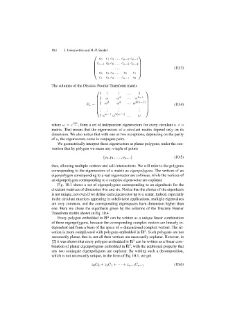
⎜ c 0 c 1 c 2 ... c n−2 c n−1 ⎟
⎜ c n−1 c 0 c 1 ... c n−3 c n−2 ⎟
⎜ ... ⎟ (10.3)
⎜ ⎟
⎝ c 2 c 3 c 4 ... c 0 c 1 ⎠
c 1 c 2 c 3 ... c n−1 c 0
The columns of the Discrete Fourier Transform matrix
⎛ ⎞
1 1 1 ... 1
⎜ 1 ω ω 2 ... ω n−1 ⎟
⎜ ⎟
⎜ 1 ω 2 ω 4 ... ω 2(n−1) ⎟
F n = ⎜ ⎟ (10.4)
⎜. . . . ⎟
⎝ . . . . . . . . ⎠
1 ω n−1 ω 2(n−1) ... ω
2πi
where ω = e n , form a set of independent eigenvectors for every circulant n × n
matrix. That means that the eigenvectors of a circulant matrix depend only on its
dimension. We also notice that with one or two exceptions, depending on the parity
of n, the eigenvectors come in conjugate pairs.
We geometrically interpret these eigenvectors as planar polygons, under the con-
vention that by polygon we mean any n-tuple of points

(p 0 ,p 1 ,...,p n−1 ) (10.5)

thus, allowing multiple vertices and self-intersections. We will refer to the polygons
corresponding to the eigenvectors of a matrix as eigenpolygons. The vertices of an
eigenpolygon corresponding to a real eigenvector are collinear, while the vertices of
an eigenpolygon corresponding to a complex eigenvector are coplanar.
Fig. 10.1 shows a set of eigenpolygons corresponding to an eigenbasis for the
circulant matrices of dimension five and six. Notice that the choice of the eigenbasis
is not unique, not even if we define each eigenvector up to a scalar. Indeed, especially
in the circulant matrices appearing in subdivision applications, multiple eigenvalues
are very common, and the corresponding eigenspaces have dimension higher than
one. Here we chose the eigenbasis given by the columns of the Discrete Fourier
Transform matrix shown in Eq. 10.4.
Every polygon embedded in R can be written as a unique linear combination
2
of these eigenpolygons, because the corresponding complex vectors are linearly in-
dependent and form a basis of the space of n-dimensional complex vectors. The sit-
uation is more complicated with polygons embedded in R . Such polygons are not
3
necessarily planar, that is, not all their vertices are necessarily coplanar. However, in
[2] it was shown that every polygon embedded in R can be written as a linear com-
3
bination of planar eigenpolygons embedded in R , with the additional property that
3
any two conjugate eigenpolygons are coplanar. By writing such a decomposition,
which is not necessarily unique, in the form of Eq. 10.1, we get
(10.6)
z 0 C 0 + z 1 C 1 + ··· + z n−1 C n−1