Page 187 - Geometric Modeling and Algebraic Geometry

10 Cube Decompositions 189
10.4 Cube decompositions

To apply the above setup to the n-dimensional cube, we first need a correspondence
n
between its vertices and the elements of Z . This can be easily done by considering
2
the unit cube. Indeed, the coordinates of its vertices are n-tuples with entries 0’s and
n
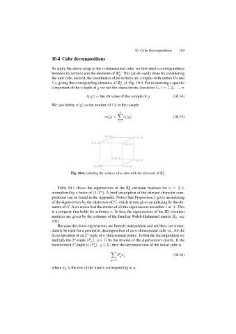
1’s, giving the corresponding elements of Z , cf. Fig. 10.4. For referencing a specific
2
component of the n-tuple of g we use the characteristic functions δ i , i =1, 2,...,n
δ i (g)= the ith value of the n-tuple of g (10.14)

We also define σ(g) as the number of 1’s in the n-tuple
n

σ(g)= δ i (g) (10.15)
i=1

Fig. 10.4. Labeling the vertices of a cube with the elements of Z 2 .
3

n
Table 10.1 shows the eigenvectors of the Z -circulant matrices for n =2, 3,
2
n
normalized by a factor of (1/2 ). A brief description of the relevant character com-
putations can be found in the Appendix. Notice that Proposition 1 gives an indexing
of the eigenvectors by the characters of G, which in turn gives an indexing by the ele-
ments of G. Also notice that the entries of all the eigenvectors are either 1 or -1. This
n
is a property that holds for arbitrary n. In fact, the eigenvectors of the Z -circulant
2
matrices are given by the columns of the familiar Walsh-Hadamard matrix H n ,see
[10].
Because the above eigenvectors are linearly independent and real they can imme-
diately be used for a geometric decomposition of an n-dimensional cube i.e., for the
n
decomposition of an 2 -tuple of n-dimensional points. To find the decomposition we
n
multiply the 2 -tuple (P g ),g ∈ G by the inverse of the eigenvector’s matrix. If the
n

transformed 2 -tuple is (P ),g ∈ G, then the decomposition of the initial cube is
g

P v g (10.16)
g
g∈G
where v g is the row of the matrix corresponding to g.