Page 190 - Geometric Modeling and Algebraic Geometry

192 I. Ivrissimtzis and H.-P. Seidel

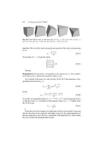
Fig. 10.7. From left to right: (a) The unit cube. (b) P 110 =(0.2, 0.0, 0.0).(c) P 110 =
(0.2, 0.2, 0.0). (d) P 110 =(0.0, 0.0, 0.2). (e) P 111 =(0.2, 0.2, 0.2).

algorithm. The row of the matrix giving the new position of the vertex corresponding
to g is
3 n−σ(g)
a g = (10.17)
4 n
For example, if n =2 we get the matrix
⎛ ⎞
9331
⎜ 3913 ⎟
⎜ ⎟ /16 (10.18)
⎝ 3193 ⎠
1339
We have

Proposition 4. The eigenvalue corresponding to the eigenvector v g of the subdivi-
sion matrix of the n-dimensional quadratic spline is 2 σ(g) .
1
For a sketch of the proof, we notice by Eq. 10.10, 10.17 the eigenvalue corre-
sponding to the character χ g is

3 n−σ(h)
= χ g (h) (10.19)
λ χ g n
4
h∈G
giving,
(3 + 1) n−σ(g) (3 − 1) σ(g)
= (10.20)
λ χ g n
4
To see this, we expand the product (3+1) n−σ(g) (3−1) σ(g) and rearrange the factors
so that the terms (3-1) are placed at the positions where δ(g)=0. Finally, from
Eq. 10.20 we get
1
= (10.21)
λ χ g
2 σ(g)
# $
In the limit, the cell converges to a single point, which is its barycenter. Assuming
that the barycenter is the origin, the limit shape is given by the eigencomponents of
the next eigenvalues, that is by the n components with eigenvalue 1/2. After scaling
the cell to counter the shrinkage effect we get