Page 191 - Geometric Modeling and Algebraic Geometry

10 Cube Decompositions 193
Proposition 5. Under multivariate quadratic B-spline subdivision the limit shape
of a cell is the sum of the eigencomponents with σ(g)=1. In particular, it is a
parallelogram for n =2 and a parallelepiped for n =3.

Similarly to the polygonal case, we can use the decomposition to find when sin-
gularities appear at the point of convergence of the initial cell. For example, in the
case n =3, if two opposite faces of the initial hexahedron have the same barycen-
ter, then the parallelepiped given by the three eigenvectors with eigenvalue 1/2 will
collapse to a parallelogram. A different type of singularity appears when the orien-
tation of one of the limit shape parallelepipeds is not consistent with the rest of the
grid. However, it should be noted that even though we can study singularities at the
barycenters of the cells, the method can not be used to deduce any analytic properties
of the limit volume, because we study the evolution of one cell in isolation.

10.5 Prism decomposition

Next we study the decomposition of a prism by the eigenvectors of the Z 2 × Z n -
circulant matrices. By Eq. 10.11 these eigenvectors are the rows of the matrix
⎡ ⎤
1 1 1 ... 1 1 1 1 ... 1
⎢ 1 ω ω 2 ... ω n−1 1 ω ω 2 ... ω n−1 ⎥
⎢ ⎥
⎢ 1 ω 2 ω 4 ... ω 2n−2 1 ω 2 ω 4 ... ω 2n−2 ⎥
⎢ ⎥
⎢ ... ... ... ... ... ... ... ... ⎥
⎢ ⎥
⎢ 1 ω n−1 ω n−2 ... ω 1 ω n−1 ω n−2 ... ω ⎥ (10.22)
⎢ ⎥
⎢ 1 1 1 ... 1 −1 −1 −1 ... −1 ⎥
⎢ ⎥
⎢ 1 ω ω 2 ... ω n−1 −1 −ω −ω 2 ... −ω n−1 ⎥
⎢ ⎥
⎣ ... ... ... ... ... ... ... ... ⎦
1 ω n−1 ω n−2 ... ω −1 −ω n−1 −ω n−2 ... −ω
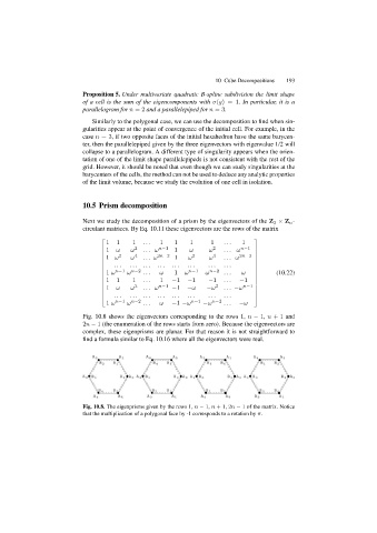
Fig. 10.8 shows the eigenvectors corresponding to the rows 1, n − 1, n +1 and
2n − 1 (the enumeration of the rows starts from zero). Because the eigenvectors are
complex, these eigenprisms are planar. For that reason it is not straightforward to
find a formula similar to Eq. 10.16 where all the eigenvectors were real.

Fig. 10.8. The eigenprisms given by the rows 1, n − 1, n +1, 2n − 1 of the matrix. Notice
that the multiplication of a polygonal face by -1 corresponds to a rotation by π.