Page 183 - Geometric Modeling and Algebraic Geometry

10 Cube Decompositions 185

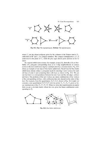
Fig. 10.1. Top: The eigenpentagons. Bottom: The eigenhexagons

where C i are the planar polygons given by the columns of the Fourier matrix F n ,
embedded in R and z i are complex numbers. The complex multiplication z i C i is
3
understood in the plane of C i , while the plus signs denote point addition in the 3d
space.
In a typical subdivision scheme, for example, Loop [12], Butterfly [13] or Doo-
Sabin [14], polygons corresponding faces or to 1-ring neighborhoods of vertices
evolve to the next subdivision step by a multiplication by a circulant matrix. Fig. 10.4
shows an example of one step of Doo-Sabin subdivision. Recall that the Doo-Sabin
subdivision scheme refines a polygonal mesh by inserting k new vertices for each
old face of order k and connecting them with faces as shown in Fig. 10.2. We can
see that there is a correspondence between the new faces and the old edges, vertices
and faces. The positions of the new vertices are linear combinations of the vertices
of the corresponding old face, with coefficients that only depend on the order of that
face. For example, from the quadrilateral P 0 P 1 P 2 P 3 shown in Fig. 10.2 (right) we

compute a new quadrilateral P P P P with the points P 0 ,P 1 ,P 2 ,P 3 given as lin-

0 1 2 3
ear combinations of the P ,P ,P ,P . When we write this transformation in matrix

0 1 2 3
form we get a circulant matrix whose first row gives the linear combination corre-
sponding to P .

0

Fig. 10.2. Doo-Sabin subdivision.