Page 37 - Geometric Modeling and Algebraic Geometry

34 F. Aries et al.
Orbit Representative

Ii 2 2 2
2 x 1x 2 :2 x 0x 2 :2 x 0x 1 : x 0 + x 1 + x 2
Iii 2 2 2

2 x 1x 2 :2 x 0x 2 :2 x 0x 1 : x 0 − x 1 + x 2
Iiii 2 2 2 2
x 0 + x 1 : x 1 + x 2 : x 0x 2 : x 1x 2

IIi 2 2 2
x 0 − x 1 : x 0x 1 : x 1x 2 : x 2
IIii 2 2 2
x 0x 2 − x 1x 2 : x 0 : x 1 : x 2
III x 0 : x 0x 2 − x 1 : x 1x 2 : x 2 2
2
2
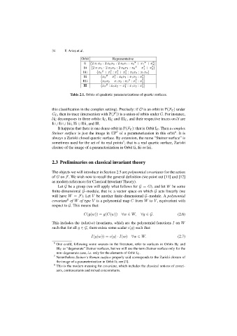
Table 2.1. Orbits of quadratic parameterizations of quartic surfaces.
this classification in the complex setting). Precisely: if O is an orbit in P(F C ) under
G C , then its trace (intersection with P(F)) is a union of orbits under G. For instance,
U C decomposes in three orbits: I C ,II C and III C , and their respective traces on U are
Ii ∪ Iii ∪ Iiii, IIi ∪ IIii, and III.
It happens that there is one dense orbit in P(F C ): that is Orbit I C . Then a complex
6
Steiner surface is just the image in CP of a parameterization in this orbit .Itis
3
always a Zariski closed quartic surface. By extension, the name “Steiner surface” is
7
sometimes used for the set of its real points ; that is a real quartic surface, Zariski
closure of the image of a parameterization in Orbit Ii, Iii or Iiii.

2.3 Preliminaries on classical invariant theory

The objects we will introduce in Section 2.5 are polynomial covariants for the action
of G on F. We wish now to recall the general definition (we point out [11] and [12]
as modern references for Classical Invariant Theory).
Let G be a group (we will apply what follows for G = G), and let W be some
finite-dimensional G–module, that is: a vector space on which G acts linearly (we
will have W = F). Let V be another finite-dimensional G–module. A polynomial
8
covariant of W of type V is a polynomial map C from W to V , equivariant with
respect to G. This means that:
C(g(w)) = g(C(w)) ∀w ∈ W, ∀g ∈G. (2.6)

This includes the (relative) invariants, which are the polynomial functions I on W
such that for all g ∈G, there exists some scalar c(g) such that:

I(g(w)) = c(g) · I(w) ∀w ∈ W. (2.7)
One could, following some sources in the literature, refer to surfaces in Orbits II C and
6
III C as “degenerate” Steiner surfaces, but we will use the term Steiner surface only for the
non–degenerate case, i.e. only for the elements of Orbit I C.
Nevertheless Steiner’s Roman surface properly said corresponds to the Zariski closure of
7
the image of a parameterization in Orbit Ii; see [7].
This is the modern meaning for covariant, which includes the classical notions of covari-
8
ants, contravariants and mixed concomitants.