Page 42 - Geometric Modeling and Algebraic Geometry

2 Some Covariants Related to Steiner Surfaces 39

a 00 a 01 a 02 2 b 00 2 b 01 2 b 02 y 0

a 10 a 11 a 12 2 b 10 2 b 11 2 b 12 y 1

1 a 20 a 21 a 22 2 b 20 2 b 21 2 b 22 y 2
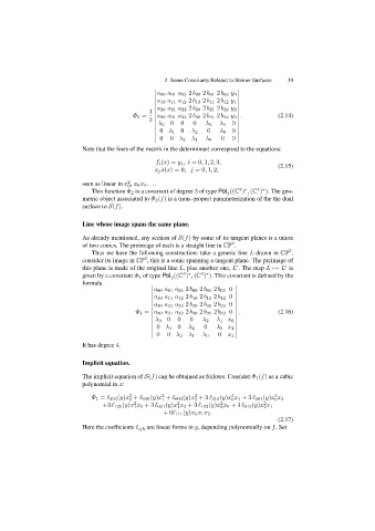
Φ 2 = a 30 a 31 a 32 2 b 30 2 b 31 2 b 32 y 3 . (2.14)

2
λ 0 0 0 0 0
λ 2 λ 1
0 λ 1 0 0 0
λ 2 λ 0
0 0 λ 2 λ 1 λ 0 0 0
Note that the lines of the matrix in the determinant correspond to the equations:
f i (x)= y i ,i =0, 1, 2, 3,
(2.15)
x j λ(x)=0,j =0, 1, 2,
seen as linear in x , x 0 x 1 , ...
2
0
4 ∗
3 ∗
This function Φ 2 is a covariant of degree 3 of type Pol ((C ) , (C ) ). The geo-
3
metric object associated to Φ 2 (f) is a (non–proper) parameterization of the the dual
surface to S(f).
Line whose image spans the same plane.
As already mentioned, any section of S(f) by some of its tangent planes is a union
of two conics. The preimage of each is a straight line in CP .
2
Thus we have the following construction: take a generic line L drawn in CP ,
2
consider its image in CP , this is a conic spanning a tangent plane. The preimage of
3
this plane is made of the original line L, plus another one, L . The map L → L is

given by a covariant Φ 3 of type Pol ((C ) , (C ) ). This covariant is defined by the
3 ∗
3 ∗
2
formula
a 00 a 01 a 02 2 b 00 2 b 01 2 b 02 0

a 10 a 11 a 12 2 b 10 2 b 11 2 b 12 0

a 20 a 21 a 22 2 b 20 2 b 21 2 b 22 0

Φ 3 = a 30 a 31 a 32 2 b 30 2 b 31 2 b 32 0 . (2.16)

λ 0 0 0 0
λ 2 λ 1 x 0
0 λ 1 0 0

λ 2 λ 0 x 1
0 0 λ 2 λ 1 λ 0 0 x 2

It has degree 4.
Implicit equation.
The implicit equation of S(f) can be obtained as follows. Consider Φ 1 (f) as a cubic
polynomial in x:
3 3 3 2 2
Φ 1 =
300 (y)x +
030 (y)x +
003 (y)x +3
210 (y)x x 1 +3
201 (y)x x 2
0 1 2 0 0
2 2 2 2
+3
120 (y)x x 0 +3
021 (y)x x 2 +3
102 (y)x x 0 +3
012 (y)x x 1
1 1 2 2
+6
111 (y)x 0 x 1 x 2 .
(2.17)
Here the coefficients
ijk are linear forms in y, depending polynomially on f. Set