Page 53 - Geometric Modeling and Algebraic Geometry

50 S. Breske et al.
This is in fact just the real and imaginary part of the first component of the general-
ized cosine h considered by Withers [21] and Chmutov [5]. It is easy to see that h 1
is a coordinate change if u − v> 0,u +2v> 0, and 2u + v< 1. It transforms the
polynomial F A 2 into the function G A 2 : 2 → 2 , defined by
,d d
G A 2 (u, v):= F A 2 (h (u, v)) = 2 cos(2πdu)+2 cos(2πdv)+2 cos(2πd(u+v))+2.
1
d ,d
The calculation of the critical points of G A 2 is exactly the same as the one performed
d
in [5]. As the function G A 2 has (d − 1) distinct real critical points in the region
2
d
defined by u − v> 0,u +2v> 0, and 2u + v< 1, the images of these points under
the map h are all the critical points of the real folding polynomial F A 2 of degree d.
1
,d
In contrast to [5], we get real critical points because h is a map from 2 into itself.
1
None of the other root systems yield more critical points on two levels. But as
mentioned in [16], the real folding polynomials associated to the root system B 2 give
n
hypersurfaces in P , n ≥ 5, which improve the previously known lower bounds for
the maximum number of nodes in higher dimensions slightly (see [16]; [3] gives a
detailed discussion of all these folding polynomials and their critical points).

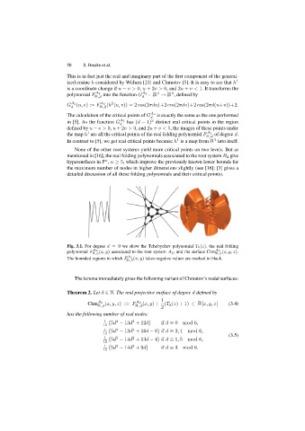
Fig. 3.1. For degree d =9 we show the Tchebychev polynomial T 9(z), the real folding
polynomial F A 2 (x, y) associated to the root system A 2, and the surface Chm A 2 (x, y, z).
,9 ,9
The bounded regions in which F A 2 (x, y) takes negative values are marked in black.
,9

The lemma immediately gives the following variant of Chmutov’s nodal surfaces:

Theorem 2. Let d ∈ N. The real projective surface of degree d defined by
1
Chm A 2 (x, y, z):= F A 2 (x, y)+ (T d (z)+1) ∈ [x, y, z] (3.4)
,d ,d
2
has the following number of real nodes:

5d − 13d +12d if d ≡ 0 mod 6,
1
2
3
12

5d − 13d +16d − 8 if d ≡ 2, 4 mod 6,
1
3
2
(3.5)
12

5d − 14d +13d − 4 if d ≡ 1, 5 mod 6,
1
2
3
12

5d − 14d +9d if d ≡ 3 mod 6.
1
2
3
12