Page 69 - Geometric Modeling and Algebraic Geometry

66 P. H. Johansen et al.
Triple point Invariants and constraints Other singularities

1 A m i −1, m i =12
T 3,3,4

T 3,3,3+m m =2,..., 12 A m i −1, m i =12 − m

2 A m i −1, m i =12
Q 10

T 9+m m =2, 3 A m i −1, m i =12 − m

3 r 0 =max(j 0,k 0), r 1 =max(j 1,k 1), A m i −1, m i =4 − k 0 − k 1,
T 3,4+r 0 ,4+r 1

j 0 > 0 ↔ k 0 > 0, min(j 0,k 0) ≤ 1, A m −1 ,

i m i =8 − j 0 − j 1
j 1 > 0 ↔ k 1 > 0, min(j 1,k 1) ≤ 1

4 S series j 0 ≤ 8, k 0 ≤ 4, min(j 0,k 0) ≤ 2, A m i −1, m i =4 − k 0,

j 0 > 0 ↔ k 0 > 0, j 1 > 0 ↔ k 0 > 1 A m −1 ,

i m i =8 − j 0
5 T 4+j k ,4+j l ,4+j m m 1 + l 1 ≤ 4, k 2 + m 2 ≤ 4, A m i −1, m i =4 − m 1 − l 1,

k 3 + l 3 ≤ 4, k 2 > 0 ↔ k 3 > 0, A m −1 , m i =4 − k 2− m 2,

i
l 1 > 0 ↔ l 3 > 0, m 1 > 0 ↔ m 2 > 0, A m −1 ,

i m i =4 − k 3 − l 3
min(k 2,k 3) ≤ 1, min(l 1,l 3) ≤ 1,
min(m 1,m 2) ≤ 1, j k = max(k 2,k 3),
j l = max(l 1,l 3), j m =max(m 1,m 2)

6 U series j 1 > 0 ↔ j 2 > 0 ↔ j 3 > 0, A m i −1, m i =4 − j 1,

at most one of j 1,j 2,j 3 > 1, A m −1 , m i =4 − j 2,

i
j 1,j 2,j 3 ≤ 4 A m −1 ,

i m i =4 − j 3
7 V series j 0 > 0 ↔ k 0 > 0, min(j 0,k 0) ≤ 1, A m i −1, m i =4 − j 0,
j 0 ≤ 4, k 0 ≤ 4

8 V series None

9 P 8 = T 3,3,3 A m i −1, m i =12
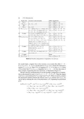
Table 4.1. Possible configurations of singularities for each case
this would imply a singular line on the monoid, so we assume that either (1 : 0 :
0) ∈ Z(f 4 ) or (1 :0:0) is a smooth point on Z(f 4 ). Let m denote the intersection
number I (1:0:0) (f 3 ,f 4 ). Since Z(f 3 ) is singular at (1 :0:0) we have m =1.From
[19] we know that O is a T 3,3,3+m singularity for m =2,..., 12. Note that some of
these complex singularities have two real forms, as illustrated in Figure 4.3.
B´ ezout’s theorem and Proposition 6 limit the possible configurations of singular-
ities on the monoid for each m. Let θ(s, t)=(−s − t ,s t, st ). Then the tangent
2
3
2
3
cone Z(f 3 ) is parameterized by θ as a map from P to P . When we need to compute
2
1
the intersection numbers between the rational curve Z(f 3 ) and the curve Z(f 4 ),we
can do that by studying the roots of the polynomial f 4 (θ). Expanding the polynomial
gives
f 4 (θ)(s, t)= a 1 s 12 − a 2 s t +(−a 3 + a 4 )s t +(4a 1 + a 5 − a 7 )s t
9 3
11
10 2
+(−3a 2 + a 6 − a 8 + a 11 )s t +(−3a 3 +2a 4 − a 9 + a 12 )s t
7 5
8 4
+(6a 1 +2a 5 − a 7 − a 10 + a 13 )s t
6 6
+(−3a 2 +2a 6 − a 8 + a 14 )s t +(−3a 3 + a 4 − a 9 + a 15 )s t
5 7
4 8
+(4a 1 + a 5 − a 10 )s t +(−a 2 + a 6 )s t − a 3 st 11 + a 1 t .
12
3 9
2 10