Page 31 - Global Tectonics

18 CHAPTER 2

depends upon their wavelength. The depth of penetra-
tion of surface waves is also wavelength-dependent,
with the longer wavelengths reaching greater depths.
Since seismic velocity generally increases with depth,
the longer wavelengths travel more rapidly. Thus,
when surface waves are utilized, it is necessary to
measure the phase or group velocities of their different
component wavelengths. Because of their low fre-
quency, surface waves provide less resolution than
body waves. However, they sample the Earth in a dif-
ferent fashion and, since either Rayleigh or Love waves
(Section 2.1.3) may be used, additional constraints on
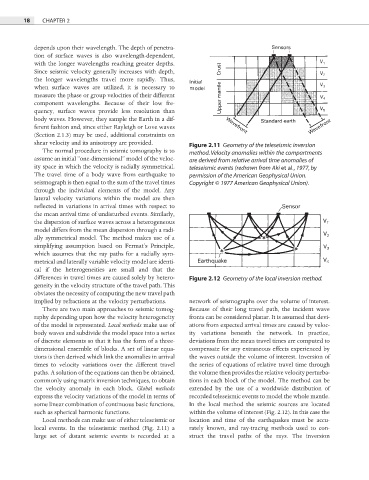
shear velocity and its anisotropy are provided. Figure 2.11 Geometry of the teleseismic inversion
The normal procedure in seismic tomography is to method. Velocity anomalies within the compartments
assume an initial “one-dimensional” model of the veloc- are derived from relative arrival time anomalies of
ity space in which the velocity is radially symmetrical. teleseismic events (redrawn from Aki et al., 1977, by
The travel time of a body wave from earthquake to permission of the American Geophysical Union.
seismograph is then equal to the sum of the travel times Copyright © 1977 American Geophysical Union).
through the individual elements of the model. Any
lateral velocity variations within the model are then

reflected in variations in arrival times with respect to
the mean arrival time of undisturbed events. Similarly,
the dispersion of surface waves across a heterogeneous
model differs from the mean dispersion through a radi-
ally symmetrical model. The method makes use of a
simplifying assumption based on Fermat’s Principle,
which assumes that the ray paths for a radially sym-
metrical and laterally variable velocity model are identi-
cal if the heterogeneities are small and that the
differences in travel times are caused solely by hetero- Figure 2.12 Geometry of the local inversion method.
geneity in the velocity structure of the travel path. This
obviates the necessity of computing the new travel path
implied by refractions at the velocity perturbations. network of seismographs over the volume of interest.
There are two main approaches to seismic tomog- Because of their long travel path, the incident wave
raphy depending upon how the velocity heterogeneity fronts can be considered planar. It is assumed that devi-
of the model is represented. Local methods make use of ations from expected arrival times are caused by veloc-
body waves and subdivide the model space into a series ity variations beneath the network. In practice,
of discrete elements so that it has the form of a three- deviations from the mean travel times are computed to
dimensional ensemble of blocks. A set of linear equa- compensate for any extraneous effects experienced by
tions is then derived which link the anomalies in arrival the waves outside the volume of interest. Inversion of
times to velocity variations over the different travel the series of equations of relative travel time through
paths. A solution of the equations can then be obtained, the volume then provides the relative velocity perturba-
commonly using matrix inversion techniques, to obtain tions in each block of the model. The method can be
the velocity anomaly in each block. Global methods extended by the use of a worldwide distribution of
express the velocity variations of the model in terms of recorded teleseismic events to model the whole mantle.
some linear combination of continuous basic functions, In the local method the seismic sources are located
such as spherical harmonic functions. within the volume of interest (Fig. 2.12). In this case the
Local methods can make use of either teleseismic or location and time of the earthquakes must be accu-
local events. In the teleseismic method (Fig. 2.11) a rately known, and ray-tracing methods used to con-
large set of distant seismic events is recorded at a struct the travel paths of the rays. The inversion