Page 87 - Glucose Monitoring Devices

86 CHAPTER 5 Modeling the SMBG measurement error

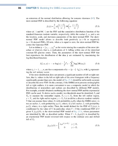
an extension of the normal distribution allowing for nonzero skewness [43]. The
skew-normal PDF is described by the following equation:

2 y x y x
f Y ðyÞ¼ $f $F a $ (5.3)
u u u
where fð $Þ and Fð $Þ are the PDF and the cumulative distribution function of the
standard Gaussian random variable, respectively, while the scalars x, u, and a are
the location, scale, and skewness parameters of the skew-normal PDF. The skew-
normal PDF model allows to describe both positively (a > 0) or negatively
(a < 0) skewed PDFs. Of note, when a is equal to zero, the skew-normal PDF be-
comes the Gaussian PDF.
T
Let us define y ¼½y 1 ; .; y n Š as the vector storing the n samples of the error (ab-
solute or relative), that is, n realizations of Y, falling within one of the identified
constant-SD glucose zones. Then, the parameters of the skew-normal PDF that
best reproduces the distribution of the data y are estimated by maximizing the
log-likelihood function:
n
1 T X
lðx; u; aÞ¼ n$logðuÞ z z logð2Fðaz i ÞÞ (5.4)
2
i¼1
where z i , i ¼ 1, ., n, are the n components of z ¼ðy x $1 n Þ=u, with 1 n represent-
ing the nx1 unitary vector.
If the error distribution does not present a significant number of left or right out-
liers, that is, values in the left or right tails of the error histogram with a frequency
significantly greater than zero, the model of Eq. (5.3) should be sufficiently accurate
to describe the error PDF. On the contrary, if the SMBG error presents nonnegligible
left or right outliers, it is more convenient to use a composite model in which the
distributions of nonoutliers and outliers are described by different PDF models.
For example, a model obtained combining the skew-normal PDF and the exponential
PDF can be used. To derive such a model, two thresholds must be identified, T 1 and
T 2 , to separate the nonoutlier region, T 1 y T 2, from the left outlier region,
y < T 1, and the right outlier region, y > T 2 . Let us define a discrete random variable
V that can assume three values: 0, with probability p V (0), when the SMBG error y is
not an outlier; 1, with probability p V (1), when y is a left outlier; 2, with probability
p V (2), when y is a right outlier. Then, the model defined for the PDF of Y, f Y (y), is
conditioned by the value of V. In particular, when V ¼ 0 the conditional PDF of Y
given V, f YjV (yj0), is the skew-normal PDF model of Eq. (5.3), whose parameters
are identified by ML as described earlier. When V ¼ 1, f YjV (yj1) is described by
an exponential PDF model reversed with respect to the ordinate axis and shifted
left of T 1 :
(
l 1 e l 1 ðyþT 1 Þ y T 1
f YjV ðyj1Þ¼ (5.5)
0 y > T 1