Page 32 - Handbook of Thermal Analysis of Construction Materials

16 Chapter 1 - Thermoanalytical Techniques

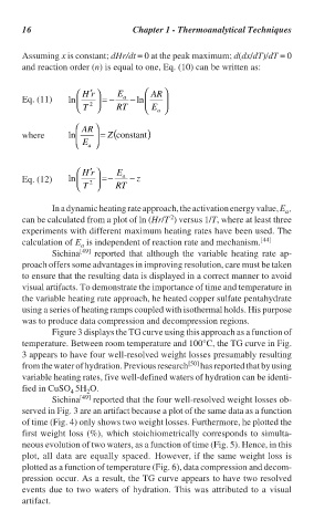
Assuming x is constant; dHr/dt = 0 at the peak maximum; d(dx/dT)/dT = 0
and reaction order (n) is equal to one, Eq. (10) can be written as:

 H ′ r  E a  AR 
Eq. (11) ln   = − − ln    
 T 2  RT  E a 

 AR 


where ln  = Z (constant )
 E a 
 H′ r  E a
Eq. (12) ln  2  = − − z
 T  RT

In a dynamic heating rate approach, the activation energy value, E ,
a
2
can be calculated from a plot of ln (Hr/T ) versus 1/T, where at least three
experiments with different maximum heating rates have been used. The
calculation of E is independent of reaction rate and mechanism. [44]
a
Sichina [49] reported that although the variable heating rate ap-
proach offers some advantages in improving resolution, care must be taken
to ensure that the resulting data is displayed in a correct manner to avoid
visual artifacts. To demonstrate the importance of time and temperature in
the variable heating rate approach, he heated copper sulfate pentahydrate
using a series of heating ramps coupled with isothermal holds. His purpose
was to produce data compression and decompression regions.
Figure 3 displays the TG curve using this approach as a function of
temperature. Between room temperature and 100°C, the TG curve in Fig.
3 appears to have four well-resolved weight losses presumably resulting
from the water of hydration. Previous research [50] has reported that by using
variable heating rates, five well-defined waters of hydration can be identi-
fied in CuSO 5H O.
4 2
Sichina [49] reported that the four well-resolved weight losses ob-
served in Fig. 3 are an artifact because a plot of the same data as a function
of time (Fig. 4) only shows two weight losses. Furthermore, he plotted the
first weight loss (%), which stoichiometrically corresponds to simulta-
neous evolution of two waters, as a function of time (Fig. 5). Hence, in this
plot, all data are equally spaced. However, if the same weight loss is
plotted as a function of temperature (Fig. 6), data compression and decom-
pression occur. As a result, the TG curve appears to have two resolved
events due to two waters of hydration. This was attributed to a visual
artifact.