Page 290 - Geology and Geochemistry of Oil and Gas

252 MATHEMATICAL MODELING IN PETROLEUM GEOLOGY

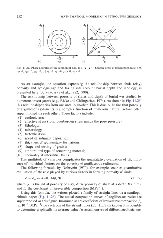
Fig. 11.24. Phase diagrams of the solution of Eqs. 11.77. I – IV – Specific areas of phase space. (a) 1 40,
2 o0, g 12 o0, g 21 40; (b) 1 40, 2 40, g 12 o0, g 21 o0.

As an example, the equation expressing the relationship between shale (clay)
porosity and geologic age and taking into account burial depth and lithology, is
presented here (Buryakovsky et al., 1982, 1990).
The relationship between porosity of shales and depth of burial was studied by
numerous investigators (e.g., Rieke and Chilingarian, 1974). As shown in Fig. 11.25,
this relationship varies from one area to another. This is due to the fact that porosity
of argillaceous sediments is a complex function of numerous natural factors, often
superimposed on each other. These factors include:
(1) geologic age;
(2) effective stress (total overburden stress minus the pore pressure);
(3) lithology;
(4) mineralogy;
(5) tectonic stress;
(6) speed of sediment deposition;
(7) thickness of sedimentary formations;
(8) shape and sorting of grains;
(9) amount and type of cementing material;
(10) chemistry of interstitial fluids.
This multitude of variables complicates the quantitative evaluation of the influ-
ence of individual factors on the porosity of argillaceous sediments.
The following formula by Dobrynin (1970), for example, enables quantitative
evaluation of the role played by various factors in forming porosity of shale:
f ¼ f expð 0:014b DÞ (11.78)
o
c
where f is the initial porosity of clay, f the porosity of shale at a depth D (in m),
o
1
and b the coefficient of irreversible compaction (MPa ).
c
Using this formula, the writers plotted a family of straight lines on a semiloga-
rithmic paper (Fig. 11.26). The actual compaction curves of argillaceous rocks are
superimposed on this figure. Inasmuch as the coefficient of irreversible compaction b c
1
3
(in 10 , MPa ) for each one of the straight lines (Eq. 11.78) is known, it is possible
to determine graphically its average value for actual curves of different geologic age: