Page 156 - Handbook of Deep Learning in Biomedical Engineering Techniques and Applications

Chapter 5 Depression discovery in cancer communities using deep learning 145

The node of RNN shown in Fig. 5.7 is a piece of neural network
model, M, which looks at some input and produces the output.
Each node in a given RNN has a self-loop that is used for remem-
bering the activation output at every time stamp. The model is
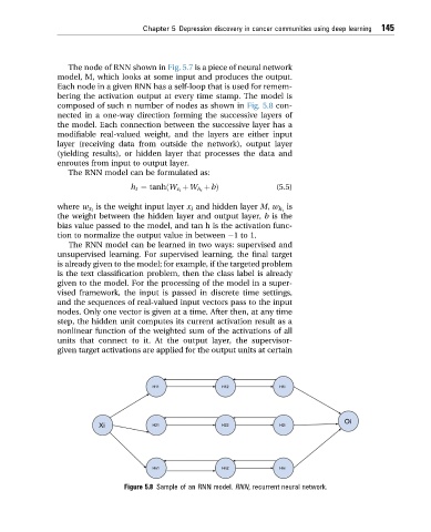
composed of such n number of nodes as shown in Fig. 5.8 con-
nected in a one-way direction forming the successive layers of
the model. Each connection between the successive layer has a
modifiable real-valued weight, and the layers are either input
layer (receiving data from outside the network), output layer
(yielding results), or hidden layer that processes the data and
enroutes from input to output layer.
The RNN model can be formulated as:

þ bÞ (5.5)
h t ¼ tanhðW x i þ W h t
is the weight input layer x i and hidden layer M, w is
where w x i
h t
the weight between the hidden layer and output layer, b is the
bias value passed to the model, and tan h is the activation func-
tion to normalize the output value in between 1to1.
The RNN model can be learned in two ways: supervised and
unsupervised learning. For supervised learning, the final target
is already given to the model; for example, if the targeted problem
is the text classification problem, then the class label is already
given to the model. For the processing of the model in a super-
vised framework, the input is passed in discrete time settings,
and the sequences of real-valued input vectors pass to the input
nodes. Only one vector is given at a time. After then, at any time
step, the hidden unit computes its current activation result as a
nonlinear function of the weighted sum of the activations of all
units that connect to it. At the output layer, the supervisor-
given target activations are applied for the output units at certain

Figure 5.8 Sample of an RNN model. RNN, recurrent neural network.