Page 39 - Hardware Implementation of Finite-Field Arithmetic

22 Cha pte r O n e

3
2
2
4
3
normal basis of F over F , because α = αα = α(α + 1) = α + α = α +
8 2
α + 1.
1.3.5 Finite Fields GF (2 )
m
Finite fields GF(2 m ) = F m are extension fields of GF (2) = F = Z . Finite
2 2 2
m
fields of order 2 are characteristic 2 finite fields, also known as binary
m
extension fields. Binary fields GF (2 ) have fundamental interest due to
thei r wide number of technical applications, such as algebraic codes,
cryptographic schemes, random number generators, digital signal processing
or VLSI testing.
m
The elements of the finite field GF (2 ) are the polynomials {0, 1,
α, α+ 1, α , α + 1, . . . , α m − 1 + α m − 2 . . . + α + 1}, where α is a root of an
2
2
+
irreducible polynomial f (x) over GF (2), f (α) = 0, and where the
polynomial coefficients are in GF (2) = {0,1}.
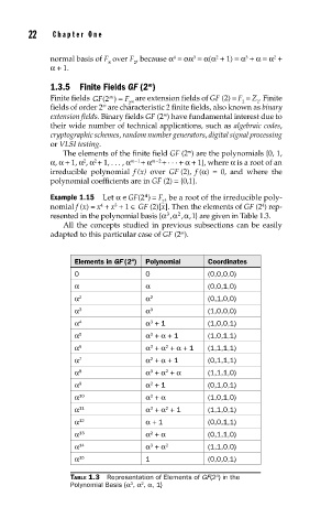
Example 1.15 Let α∈GF() = F 4 be a root of the irreducible poly-
2
4
2
4
4
3
nomial f (x) = x + x + 1 ∈ GF (2)[x]. Then the elements of GF (2 ) rep-
resented in the polynomial basis {αα 2 , , } are given in Table 1.3.
α
3
1
,
All the concepts studied in previous subsections can be easily
adapted to this particular case of GF (2 ).
m
4
Elements in GF (2 ) Polynomial Coordinates
0 0 (0,0,0,0)
α α (0,0,1,0)
α 2 α 2 (0,1,0,0)
α 3 α 3 (1,0,0,0)
α 4 α + 1 (1,0,0,1)
3
α 5 α +α+ 1 (1,0,1,1)
3
α 6 α +α +α+ 1 (1,1,1,1)
3
2
α 7 α +α+ 1 (0,1,1,1)
2
α 8 α +α +α (1,1,1,0)
3
2
α 9 α + 1 (0,1,0,1)
2
α 10 α +α (1,0,1,0)
3
α 11 α +α + 1 (1,1,0,1)
2
3
α 12 α+ 1 (0,0,1,1)
α 13 α +α (0,1,1,0)
2
α 14 α +α 2 (1,1,0,0)
3
α 15 1 (0,0,0,1)
4
TABLE 1.3 Representation of Elements of GF(2 ) in the
2
3
Polynomial Basis {α , α , α, 1}