Page 43 - Hardware Implementation of Finite-Field Arithmetic

26 Cha pte r T w o

r
y
q = –1 q = 0 q = 1

s
–2y –y y 2y

–y
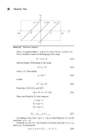
FIGURE 2.1 Robertson diagram.

Thus, r is equal to either s − y (if q = 1), s (if q = 0), or s + y (if q = −1).
Now consider a natural m belonging to the range

k
2 k − 1 ≤ m < 2 (2.2)
and an integer x belonging to the range
n
−2 ≤ x < 2 n (2.3)
with n ≥ k. Then define
y = m2 n − k (2.4)
so that

n
2 n − 1 ≤ y < 2 (2.5)
From Eqs. (2.3), (2.4), and (2.5)

−2y ≤ −2 ≤ x < 2 ≤ 2y (2.6)
n
n
Then, use Property 2.1 and compute
x = q y + r
1 1
2r = q y + r
1 2 2
2r = q y + r
2 3 3
. . .
2r = q y + r (2.7)
n − k n − k + 1 n − k + 1
According to Eq. (2.6), −2y ≤ x < 2y, so that Property 2.1 can be
used and −y ≤ r < y.
1
Similarly, as −2y ≤ 2r < 2y Property 2.1 can be used and −y ≤ r < y,
1 2
and so on. To summarize
−y ≤ r < y, ∀i = 1, 2, . . . , n − k + 1 (2.8)
i