Page 98 - Hardware Implementation of Finite-Field Arithmetic

mod m Operations 81

parallel_register: process(clk)
begin
if clk’event and clk = ‘1’ then
if load = ‘1’ then pc <= (others => ‘0’);
ps <= (others => ‘0’);
elsif ce_p = ‘1’ then pc <= next_pc; ps <= next_ps;
end if;
end if;
end process parallel_register;
shift_register: process(clk)
begin
if clk’event and clk = ‘1’ then
if load = ‘1’ then int_x <= x;
elsif ce_p = ‘1’ then
for i in 0 to K-2 loop int_x(i) <= int_x(i+1);
end loop;
int_x(K-1) <= ‘0’;
end if;
end if;
end process shift_register;
xi <= int_x(0);
The complete model additionally includes the circuits corre-
sponding to the final steps, that is,

p <= ps + pc;
p_minus_m <= p + minus_m;
with p_minus_m(K) select z <= p(K-1 downto 0) when ‘0’,
p_minus_m(K-1 downto 0) when others;

as well as a k-state counter and a control unit. As regards the done
variable, a comment similar to Comment 2.1 must be done.

3.4.4 Comparison
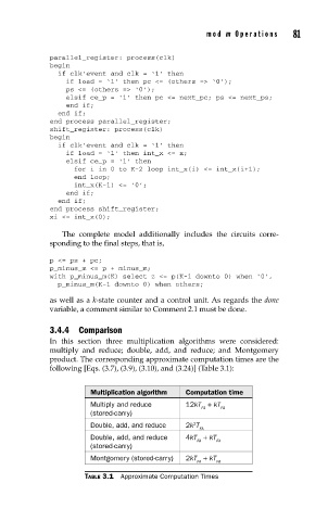
In this section three multiplication algorithms were considered:
multiply and reduce; double, add, and reduce; and Montgomery
product. The corresponding approximate computation times are the
following [Eqs. (3.7), (3.9), (3.10), and (3.24)] (Table 3.1):

Multiplication algorithm Computation time
Multiply and reduce 12kT + kT
FA FA
(stored-carry)
2
Double, add, and reduce 2k T
FA
Double, add, and reduce 4kT + kT
FA FA
(stored-carry)
Montgomery (stored-carry) 2kT + kT
FA FA
TABLE 3.1 Approximate Computation Times